お久しぶりです、Webエンジニアの本間です。
去る2019年10月1日に自分が所属するチームで担当した「ルクミーフォト」のリニューアル版をリリースすることができました。
【プレスリリース】『ルクミーフォト』および ユニファコーポレートサイトリニューアル


今回、こちらのリニューアルで技術的にどのような変更があったのか、その変更はどういう意図を持って実施したのか、広く浅めに紹介したいと思います。
続きを読むお久しぶりです、Webエンジニアの本間です。
去る2019年10月1日に自分が所属するチームで担当した「ルクミーフォト」のリニューアル版をリリースすることができました。
【プレスリリース】『ルクミーフォト』および ユニファコーポレートサイトリニューアル


今回、こちらのリニューアルで技術的にどのような変更があったのか、その変更はどういう意図を持って実施したのか、広く浅めに紹介したいと思います。
続きを読むBy Matthew Millar R&D Scientist at ユニファ
This is part IV of the MAG (Multi-Model Attribute Generator) paper I am working on. This post will start to look at the clothing color of the upper body and the lower body with different models for each (but, with the same architecture). So, for a recap of the previous post, we have completed a gender identifier Multi-Model Attribute Generator - ユニファ開発者ブログ
We have created both upper and lower body clothing classifiers
MAG part II - ユニファ開発者ブログ
MAG Part III Upper Body - ユニファ開発者ブログ
And now we are turning to color descriptors. The color that will be looked at is the primary colors of; Red, White, Yellow, Green, Purple, Blue, and Black for the upper body. The primary colors for the lower body will be; Brown, Red, White, Yellow, Green, Grey, Blue, and Black.
These colors were chosen as they are the primary colors that appeared on the upper and lower bodies of most people in the dataset. These selected colors are by far not a full representation of every possible color possible but are a good sample of many people. Some colors like pink and teal are rolled into red and blue respectively. This was done as there were not enough images with teal or pink in the dataset to make a whole new class. There should be a set of 400 or more images to make a class which was the cut off number for each color.
Seeing that the goal of the product is not necessarily an object identification but a color I turned to the literature to give me good architecture. I copied a similar architecture to the paper Vehicle Color Recognition using Convolutional Neural Network (Rachmadi & Purnama, 2015) https://arxiv.org/abs/1510.07391. This paper performed well, and the architecture does well for classifying color. Choosing a different architecture from my previous post was necessary as I was trying to get color rather than features from each image. So, the use of a fine turned Xeception model or ResNet50 model would not be ideal in this situation. This is the reason why I chose to create another model from scratch and not extend or fine-tune a pre-trained model.
The CNN for this model consists of two networks. Each of these base networks has 8 layers. The basic conv block is a convolutional layer followed by a normalization and pooling layers. Then the use of Relu as an activation for each layer is used. There are 5 different convolutional layers in the base network. For more information about the network see the above-mentioned paper. I will not go into the details of the model as the paper describes it very well.
This is the code for the CNN architecture. It looks more complicated than the previous post, but this is because of it not using a pre-trained model for the backbone.
def net(num_classes):

    input_image = Input(shape=(224,224,3))
    x = Convolution2D(filters=48,kernel_size=(11,11),strides=(4,4),
                              input_shape=(224,224,3),activation='relu')(input_image)
    top_x_1 = BatchNormalization()(top_x_1)
    top_x_1 = MaxPooling2D(pool_size=(3,3),strides=(2,2))(top_x_1)
    top_x_2 = Lambda(lambda x : x[:,:,:,:24])(top_x_1)
    bot_x_2 = Lambda(lambda x : x[:,:,:,24:])(top_x_1)

    top_x_2 = Convolution2D(filters=64,kernel_size=(3,3),strides=(1,1),activation='relu',padding='same')(top_x_2)
    top_x_2 = BatchNormalization()(top_x_2)
    top_x_2 = MaxPooling2D(pool_size=(3,3),strides=(2,2))(top_x_2)

    bot_x_2 = Convolution2D(filters=64,kernel_size=(3,3),strides=(1,1),activation='relu',padding='same')(bot_x_2)
    bot_x_2 = BatchNormalization()(bot_x_2)
    bot_x_2 = MaxPooling2D(pool_size=(3,3),strides=(2,2))(bot_x_2)
    top_x_3 = Concatenate()([top_x_2,bot_x_2])
    top_x_3 = Convolution2D(filters=192,kernel_size=(3,3),strides=(1,1),activation='relu',padding='same')(top_x_3)

    top_x_4 = Lambda(lambda x : x[:,:,:,:96])(top_x_3)
    bot_x_4 = Lambda(lambda x : x[:,:,:,96:])(top_x_3)

    top_x_4 = Convolution2D(filters=96,kernel_size=(3,3),strides=(1,1),activation='relu',padding='same')(top_x_4)
    bot_x_4 = Convolution2D(filters=96,kernel_size=(3,3),strides=(1,1),activation='relu',padding='same')(bot_x_4)

    top_x_5 = Convolution2D(filters=64,kernel_size=(3,3),strides=(1,1),activation='relu',padding='same')(top_x_4)
    top_x_5 = MaxPooling2D(pool_size=(3,3),strides=(2,2))(top_x_5)

    bot_x_5 = Convolution2D(filters=64,kernel_size=(3,3),strides=(1,1),activation='relu',padding='same')(bot_x_4)
    bot_x_5 = MaxPooling2D(pool_size=(3,3),strides=(2,2))(bot_x_5)

    bottom_x_1 = Convolution2D(filters=48,kernel_size=(11,11),strides=(4,4),
                              input_shape=(227,227,3),activation='relu')(input_image)
    bottom_x_1 = BatchNormalization()(bottom_x_1)
    bottom_x_1 = MaxPooling2D(pool_size=(3,3),strides=(2,2))(bottom_x_1)

    bottom_x_2 = Lambda(lambda x : x[:,:,:,:24])(bottom_x_1)
    bottom_bot_x_2 = Lambda(lambda x : x[:,:,:,24:])(bottom_x_1)

    bottom_x_2 = Convolution2D(filters=64,kernel_size=(3,3),strides=(1,1),activation='relu',padding='same')(bottom_x_2)
    bottom_x_2 = BatchNormalization()(bottom_x_2)
    bottom_x_2 = MaxPooling2D(pool_size=(3,3),strides=(2,2))(bottom_x_2)

    bottom_bot_x_2 = Convolution2D(filters=64,kernel_size=(3,3),strides=(1,1),activation='relu',padding='same')(bottom_bot_x_2)
    bottom_bot_x_2 = BatchNormalization()(bottom_bot_x_2)
    bottom_bot_x_2 = MaxPooling2D(pool_size=(3,3),strides=(2,2))(bottom_bot_x_2)

    bottom_x_3 = Concatenate()([bottom_x_2,bottom_bot_x_2])
    bottom_x_3 = Convolution2D(filters=192,kernel_size=(3,3),strides=(1,1),activation='relu',padding='same')(bottom_x_3)

    bottom_x_4 = Lambda(lambda x : x[:,:,:,:96])(bottom_x_3)
    bottom_bot_x_4 = Lambda(lambda x : x[:,:,:,96:])(bottom_x_3)

    bottom_x_4 = Convolution2D(filters=96,kernel_size=(3,3),strides=(1,1),activation='relu',padding='same')(bottom_x_4)
    bottom_bot_x_4 = Convolution2D(filters=96,kernel_size=(3,3),strides=(1,1),activation='relu',padding='same')(bottom_bot_x_4)

    bottom_x_5 = Convolution2D(filters=64,kernel_size=(3,3),strides=(1,1),activation='relu',padding='same')(bottom_x_4)
    bottom_x_5 = MaxPooling2D(pool_size=(3,3),strides=(2,2))(bottom_x_5)

    bottom_bot_x_5 = Convolution2D(filters=64,kernel_size=(3,3),strides=(1,1),activation='relu',padding='same')(bottom_bot_x_4)
    bottom_bot_x_5 = MaxPooling2D(pool_size=(3,3),strides=(2,2))(bottom_bot_x_5)

    output_x = Concatenate()([top_x_5,bot_x_5,bottom_x_5,bottom_bot_x_5])

    flatten = Flatten()(output_x)

    # Fully-connected layer
    FC_1 = Dense(units=4096, activation='relu')(flatten)
    FC_1 = Dropout(0.6)(FC_1)
    FC_2 = Dense(units=4096, activation='relu')(FC_1)
    FC_2 = Dropout(0.6)(FC_2)
    output = Dense(units=num_classes, activation='softmax')(FC_2)

    model = Model(inputs=input_image,outputs=output)
    sgd = SGD(lr=1e-3, decay=1e-6, momentum=0.9, nesterov=True)
    model.compile(optimizer=sgd, loss='categorical_crossentropy', metrics=['accuracy'])

    return model
This is followed by the Image generators for the training and validation sets. Nothing we have not seen before
train_datagen = ImageDataGenerator( rescale=1./255,
                                   shear_range=0.2,
                                   zoom_range=0.3,
                                   horizontal_flip=True,
                                   validation_split=0.20) # set validation split

train_generator = train_datagen.flow_from_directory(
    Data_Dir,
    target_size = (224, 224),
    shuffle=True,
    batch_size=BATCH_SIZE,
    class_mode='categorical',
    subset='training') # set as training data

validation_generator = train_datagen.flow_from_directory(
    Data_Dir, # same directory as training data
    target_size = (224, 224),
    batch_size=BATCH_SIZE,
    shuffle= False,
    class_mode='categorical',
    subset='validation') # set as validation data
And then the fitting and testing of the model:
history = model.fit_generator(
    train_generator,
    steps_per_epoch = train_generator.samples//BATCH_SIZE,
    validation_data = validation_generator,
    validation_steps = validation_generator.samples//BATCH_SIZE,
    epochs = EPOCHS,
    verbose=1,
    callbacks=callbacks_list)
The results are very results are fairly good here. Looking at the confusion metrics, most of the images are classified correctly. The two colors with the biggest issue are white as it seems to be predicted as red and yellow, and black. This might be due to striped shirts, images that are blurry, or images that are not centered on the shirt and have a lot of background in them. White might just be close enough to pink and lime green to be classified as those colors.
Classification Report
              precision    recall  f1-score   support

       Brown       0.63      0.74      0.68        86
         Red       0.66      0.68      0.67        81
       White       0.51      0.65      0.57        81
      Yellow       0.55      0.70      0.61        33
       Green       0.46      0.57      0.51        79
        Grey       0.75      0.35      0.48        77
        Blue       0.82      0.66      0.73        82
       Black       1.00      0.40      0.57        20

    accuracy                           0.61       539
   macro avg       0.67      0.59      0.60       539
weighted avg       0.65      0.61      0.61       539
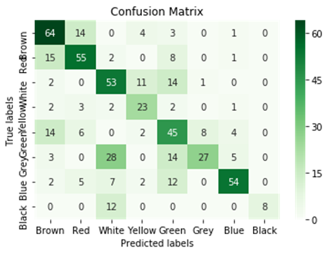
For the lower body, the results were ok. This might be due to many people wearing shorts and the existence of bags or the background changing dramatically in several of the photos. This could result in a loss of accuracy and recall for each color. Black and grey seem to be the hardest colors for the model to detect and classify correctly. This makes me think that the background is a larger problem for the lower body parts. Grey got miss classified as green and white mostly. The largest question is why black is missing classified as white. This I feel is related mostly to people wearing shorts in the dataset or white/black shirts that overlap in the image.
Classification Report
              precision    recall  f1-score   support

       Brown       0.63      0.74      0.68        86
         Red       0.66      0.68      0.67        81
       White       0.51      0.65      0.57        81
      Yellow       0.55      0.70      0.61        33
       Green       0.46      0.57      0.51        79
        Grey       0.75      0.35      0.48        77
        Blue       0.82      0.66      0.73        82
       Black       1.00      0.40      0.57        20

    accuracy                           0.61       539
   macro avg       0.67      0.59      0.60       539
weighted avg       0.65      0.61      0.61       539

So, this different CNN architecture does work quite well for color extraction. I will have to go back to the model and fine-tune the data and the model to try to rise the recall rate on white and black, but for the rest of the colors, the results are fine. This current architecture will work fine for the lower body color as there are fewer colors and won't have many shades or hues.
Rachmadi, R. F., Purnama, K. E., (2015) Vehicle Color Recognition using Convolutional Neural Network arXiv:1510.07391 [cs.CV]
おはようございます、こんにちは、こんばんは! ユニファのインフラ見てますすずきです。
エンジニアメンバーが増えて久々の更新となります。 その間にインフラメンバーも増えて新たなチャレンジがしやすい状況となってきました。
そういう状況だからと言うわけではないですが、ServerlessDays Tokyo 2019にスポンサーさせていただきました。
去年は個人スポンサーとしてServerlssConfに参加しましたが、今年は企業スポンサーでブース参加です。
1週間ほど時間が空きましたがその内容をブログに書こうと思います。
続きを読むBy Matthew Millar R&D Scientist at ユニファ
This is part III of the MAG (Multi-Model Attribute Generator) paper I am working on. This post will focus on defining what clothing the upper half of a person is wearing. As with the last post, this will not look at color right now as that will follow later. This model will allow for the classification of two different clothing types; long sleeves, and short sleeves. This model will conclude the classification of the clothing that is being worn by a person.
PART I: Multi-Model Attribute Generator - ユニファ開発者ブログ
PART II: MAG part II - ユニファ開発者ブログ
Looking at the failures and successes of the Lower body discriminator, we can apply this knowledge to make a better model quicker and more accurate.
One issue of the last post was the difficulty of knowing if a person is wearing shorts or pants. There were a lot of miss classifications due to the data sorting criteria that I used. To fix this issue, a "hard choice" criterion was made to limit this issue in the upper body model. Now, if any skin is shown, it will be considered a short sleeve shirt. However, this is not ideal as some people will roll up their sleeves which did exist in the new dataset. These cases were discarded as it would cause issues in the model's training. This might be a problem as they are truly wearing long sleeve shirts. However, due to the selection/sorting criteria, they are wearing short sleeve shirts and thus could not be included in the long sleeve shirt dataset. By doing this, it will limit the misclassification that occurred due to the high-water pants and long shorts issue in the previous post. This is an acceptable approach because using this model as a ReID attribute generator, rolled up sleeve can be considered short sleeves due to the nature of its position on the arm. Thus passing the logical "Duck Test".
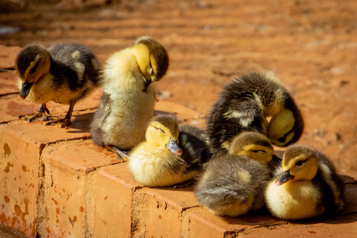
If it looks like a duck, swims like a duck, and quacks like a duck, then it probably is a duck.
Ok so for long and short sleeves, the Market1501 dataset is not sufficient as there are no long sleeve shirts in the dataset. So, I had to bring in another ReID dataset called CUHK01 (Li et.al., 2014). This is a very similar dataset and is often used in the same study as an alternative or extra data. This makes the use of this dataset for long sleeves an acceptable alternative/addition to the Market1501 dataset.
Now that this is another binary problem, it will be very similar to the gender classifier we built in part 1 (See above link). To make this simple we will just borrow the new version of the Gender Classification model. This way we know it should work well because for this as long and short sleeves are easier to tell apart than gender.
def build():
    img = Input(shape=(224,224,3))
    # Get the base of the image
    x = base_extractor(img)
    print(x.shape)

    x = Dense(2048, activation='relu')(x)
    x = Dense(2048, activation='relu')(x)
    x = Dropout(0.3)(x)
    x = BatchNormalization()(x)
    x = Dense(2048, activation='relu')(x)
    x = Dense(2048, activation='relu')(x)
    x = Dropout(0.3)(x)
    x = BatchNormalization()(x)

    pred = Dense(1, activation='sigmoid')(x)
    return Model(inputs = img, outputs = pred)
The data set up will be much the same as the lower body classifier as we are only interested in the upper portion of the body. We can use a slightly modified image cropper from the lower body model.
def crop_upper_part(img):
    y,x,_ = img.shape
    startx = 0
    starty = 0
    return img[starty:y//2,startx:startx+x]

def crop_generator(batches):
    while True:
        batch_x, batch_y = next(batches)
        batch_crops = np.zeros((batch_x.shape[0], 112, 224, 3))
        for i in range(batch_x.shape[0]):
            batch_crops[i] = crop_upper_part(batch_x[i])
        yield (batch_crops, batch_y)
The rest of the model follows a typical set up. So, I will not go into it but will just leave it here for you if you want it.
EPOCHS = 10
LR = 0.001
opt = SGD(lr=LR, momentum=0.9, decay=LR / EPOCHS)
model = build()
model.compile(loss="binary_crossentropy",
              optimizer=opt,
              metrics=["accuracy"])
filepath= "LongShort-{epoch:02d}-{val_accuracy:.4f}.h5"
checkpoint = ModelCheckpoint(filepath, monitor='val_accuracy', verbose=1, save_best_only=True, mode='max', save_weights_only=False)

reduce_lr = ReduceLROnPlateau(monitor='val_loss', factor=0.2, patience=1, min_lr=0.0001)

callbacks_list = [checkpoint,reduce_lr]

history = model.fit_generator(
    train_generator,
    steps_per_epoch = train_generator.samples // BATCH_SIZE,
    validation_data = validation_generator,
    validation_steps = validation_generator.samples // BATCH_SIZE,
    epochs = EPOCHS,
    verbose=1,
    callbacks=callbacks_list)
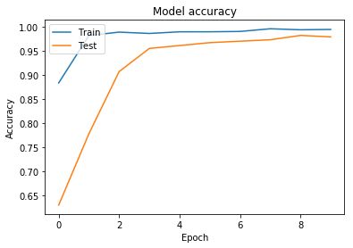
The results are very good. Looking at the accuracy is very good with a score and accuracy for evaluation of
[0.00686639454215765, 0.9836065769195557]
Looking at the confusion matrix, the model performs up to par and then some.
Confusion Matrix
[[181   3]
 [  3 179]]
Classification Report
              precision    recall  f1-score   support

       Short       0.98      0.98      0.98       184
        Long       0.98      0.98      0.98       182

    accuracy                           0.98       366
   macro avg       0.98      0.98      0.98       366
weighted avg       0.98      0.98      0.98       366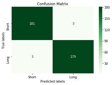
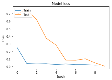
So, this model has performed stellar. Why is that, well from the lessons I have learned as I was building out the other two models. I used what worked and discarded what didn’t.
By using a finetuned pre-trained model, the accuracy automatically gets a boost for this dataset. By cropping the image to only what I want the model to learn has greatly increased the accuracy. And keeping the preprocessing of each image the same and the fine-tuned model in every single other model makes sure there are not issues in data preparation. This also future proofs these models so I know that they will work together in the final product.
Join me next time when we will start on the color of the upper body.
W. Li, R. Zhao, T. Xiao and X. Wang, "DeepReID: Deep Filter Pairing Neural Network for Person Re-identification," 2014 IEEE Conference on Computer Vision and Pattern Recognition, Columbus, OH, 2014, pp. 152-159.
doi: 10.1109/CVPR.2014.27
Image from https://www.pexels.com/search/duck/
こんにちは、iOSエンジニアのしだです。
開発ブログは久々な気がします。今回は TensorFlow Serving のgRPCの簡単な負荷試験してみます。
ECS などで TensorFlow Serving を運用する際に、どれくらいのマシンリソースだとどれくらい処理できるということを確認するためにやってます。
TensorFlow Serving はTensorFlowの学習済みのモデルをAPI化したいときに便利です。 Flaskなどで独自にWebサーバーを用意しなくてもSavedModelを用意するだけでAPIとして提供できます。 負荷試験ツールは ghz というフレームワークを利用します。
TensorFlow Serving のDockerイメージが提供されているので、それと学習済みの物体検出モデルを使ってAPIを用意します。 そして ghz を使って gRPC の負荷試験できるようにローカルで動かすまでやりたいと思います。
続きを読むみなさんこんにちは。ユニファでCTOをしてます赤沼です。先日 AWS さん主催の招待制オフサイトカンファレンス CTO Night & Day に参加させていただきました。昨年初めて参加させていただいて今回で2回目だったのですが、名だたる企業の大先輩CTOや、同じような規模・フェーズのスタートアップのCTOまで100人以上が参加していて、セッションの内容だけでなくネットワーキングやディスカッションの時間も多く、とても学びの多い2日間でした。全ての内容について書くと長くなりすぎてしまうので、その中で特に学びのあったことなどについて書きたいと思います。


今回参加するにあたって自分なりに特に何か気づきを得たいと思っていたこととして、「CTOとしての経営への関わり方」をテーマとしていました。もともと技術畑でエンジニアをしていた自分としては、取締役として経営に関わっていく中で、技術やプロダクト、ビジネス、ファイナンスなどにおいて、どのようなバランスでどのように価値を出していくかを悩んでいるところでもあり、セッションやディスカッションの中で他社の CTO の方々がどのように取り組まれているのかを参考にさせていただき、自分なりの気づきを得たいと思っていました。
そんなところにうってつけだったのが、今回アンカンファレンスのテーマの一つであった「経営者としてCTOがすべきこと」。6〜7人で一つのグループを作りディスカッションするという形で、私もこのディスカッションに参加させていただきました。その中でたまたま VOYAGE GROUP の CTO の小賀さんとご一緒させていただいたのですが、もっとも考えさせられたのが冒頭で小賀さんが投げかけられた「みなさん経営してますか?」という問いでした。経営にどう関わるかという視点はあったものの、そもそも経営とはなんなのかという点は深く突き詰めたことはなかったので、これが自分なりにでも定まっていないとどう関わっていくかもはっきりしてこないなと。また、その後のディスカッションの中でも小賀さんからお話いただいた、ビジネスやファイナンスにおいてCTOがどのように関わっていくかという点でも、やはりまず経営をする立場という点を考えれば、技術的な内容だけでなく、ビジネスやファイナンスについても勉強しておく必要があり、他の CxO に技術的な内容を話していく上でも、共通言語としてビジネスやファイナンスを学んだ上で、理解してもらえる形で話していく必要があるという点も自分として今後強く意識していこうと思った内容でした。
2日間のプログラムの最後として行われたこのセッションは、Keynote等で登壇した CTO(メルカリ 名村さん、Sansan 藤倉さん、 グリー 藤本さん、DMM 松本さん、SORACOM 安川さん、カーディナル 安武さん)が会場からの sli.do での質問にどんどん答えていくというものでした。テーマは特に限定されていないので様々な質問がありましたが、その中で、どんな質問だったかは失念しましたが、安武さんが回答されていた「経営者であれば経営に必要なことはなんでもやって当然」というような内容はとても印象に残るものでした。CTOとしてはどうしても技術的な領域のみに関わる意識になってしまいがちなのですが、CTOである以前に経営陣の1人であると考えれば、領域にとらわれることなく、必要なことはなんでもやって当然と改めて考え直させられるものでした。
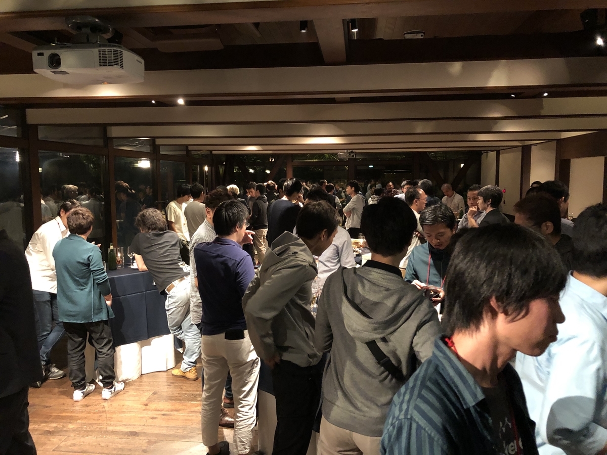
CTO Dojo というコーナーでは事前に登壇者の募集があり、私も応募させていただきまして、「開発チーム 1人 -> 40人 になるまでにやってきたこと」というタイトルで、私が1人目の正社員エンジニアとしてユニファに入社して、現在40名ほどの開発チームになるまでに取り組んできたことについてお話させていただきました。オーディエンスもみなさんCTOということで、なかなか緊張する場ではありましたが、多くの方に参加いただき、共感いただいた方も多かったようです。その後の懇親会等でもお声がけいただくこともあり、やっぱり発表する場があるなら発表しておくものだなと思った次第です。
セッションの中でもご紹介させていただいたユニファの Podcast や Meetup 等、ゲスト参加や合同開催に興味のある方はぜひお声がけいただければと思います。
ここまでに書いたセッション以外にも、オムロンさんにお邪魔してSINIC理論のワークショップに参加させていただいたり、グローバルスタートアップのCxOの Keynote があったり、1日目の夜のパーティーはなかなかすごかったりと中身の濃い二日間でした。また、私の今回のテーマに関するところでも、公開CTOメンタリングでの DMM 松本さんや CTO Dojo での freee 横路さんのお話を聞いていて、ビジネスについてもしっかり数字で語れるという点は自分にも必要だなと思った点です。
それと改めて、今回お話させていただいた方やセッションに参加いただいた方、運営いただいたAWSの皆さま、ありがとうございました。また来年お声がけいただけましたら、ぜひ参加させていただき、今回と比べて自分がアップデートできていると思えるように取り組んで行きたいと思います。


ユニファでは開発メンバーも募集してますのでご興味ある方はぜひどうぞ!!
By Matthew Millar R&D Scientist at ユニファ
This is part II of the MAG (Multi-Model Attribute Generator) paper I am working on. You can see part 1 here
Multi-Model Attribute Generator - ユニファ開発者ブログ
This post will focus on defining what clothing the lower half of a person is wearing. This will not look at color right now as that will follow in the next few posts. This model will allow for the classification of three different clothing types; skirts/dresses, shorts, and pants.
So, from my previous post, I was only getting around 56% accuracy which is ok but not good enough. I altered my code to use a fine turned Xception model trained on the Market1501 dataset. I then used this as the base feature extractor which gave very good results in Keras. My experiments showed that the Resent50 did not produce as good results compared to Xception pre-trained models for this dataset. The data argumentation consists of rotation, cropping, vertical and horizontal shifts, and horizontal flipping. I also added a preprocessing script into the data augmentation which processes each image using the Xception preprocessing input which greatly helps in the accuracy of the model as well as keeping the handling of input consistent between this model and the base model as the Xception preprocessing was performed there as well. This aids in keeping the handling of input consistent between models and limits errors that could occur due to inconsistent preprocessing.
The first step is to separate the images into their classes for Keras to use in the data generator. This will consist of three classes, Dress/skirts, shorts, and pants.
The next step is to create the base feature extractor by importing the pre-trained model and creating a new base model using Keras Function API.
base_model = load_model('pre_trained_model.ckpt')
base_extractor = Model(inputs=base_model.input, outputs=base_model.get_layer('glb_avg_pool').output)
for layer in base_extractor.layers:
    layer.trainable = True
Note the output should be the last layer before the Softmax Fully connected layer. This will give you a feature vector over a prediction.
This will prime the base model to be used for the feature extractor. Remember you want to set each layer to trainable to allow for the base model to be retrained for the specific task. The next step is to actually build out the new model for classification.
def build():
    img = Input(shape=(224,224,3))
    # Get the base of the image
    x = base_extractor(img)
    x = Dense(2048, activation='relu')(x)
    x = Dropout(0.2)(x)
    x = Dense(2048, activation='relu')(x)
    x = Dropout(0.2)(x)
    x = BatchNormalization()(x)
    print(x.shape)
    pred = Dense(3, activation='sigmoid')(x)
    return Model(inputs = img, outputs = pred)
Seeing that we are only looking at the lower portion of the body we will need to crop the image using a custom image generator.
# Custom cropping method for preprocessing
def crop_lower_part(img):
    # xception preprocessing an image should be called in the datagen not here in the prefrocess function
    y,x,_ = img.shape
    startx = 0
    starty = y//2
    return img[starty:y,startx:startx+x]

def crop_generator(batches):
    while True:
        batch_x, batch_y = next(batches)
        batch_crops = np.zeros((batch_x.shape[0], 112, 224, 3))
        for i in range(batch_x.shape[0]):
            batch_crops[i] = crop_lower_part(batch_x[i])
        yield (batch_crops, batch_y)
This basically cuts the image in half (the lower portion only) and create new images and send the batch to the model when needed.
We will be using binary cross-entropy over the categorical version for multi-label classification. This can be confusing as most every other model out there uses a categorical version. However, this works by treating each output label as an independent Bernoulli distribution which gives greater accuracy over the traditional approach (Hazewinkel, 2001). This will allow for each output node to be singularly penalized for the wrong answer. Which should in return give better more accurate results overall.
While categorical_crossentropy was getting 75% was decent results, by using binary_crossentropy over categorical_crossentropy, the accuracy increased by 5%. 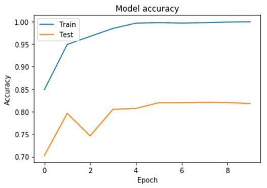
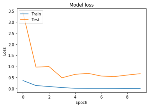
We are still overfitting after the 5 epoch, but this might be managed by cleaning the dataset by adding more samples as well as making a clear definition between shorts and pants as some samples of shorts look very close to pants. For example, some men's shorts are very long and some women's pants are higher which will look the same to the model. So this might be a battle between high water pants and long shorts.
| HighWater Pants | Long Shorts | |
 |
 |
Keras score and accuracy for the model look pretty good.
So for target T and network output O, the binary_crossentropy is:
f(T,O) = -(T*log(O) + (1-T)*log(1-O) )
And this model's score and accuracy are:
[0.19746318459510803, 0.8602761030197144]
The score is the evaluation of the loss for a given input. and the accuracy is how accurate the model is for a given input. The lower the score the better and the higher the accuracy the better.
The final evaluation of the results came back pretty decent. The accuracy of the model is about 86% for the evaluation dataset.
We saw some significant improvement in accuracy by using a pre-trained fine-tuned model that works well with Keras. The model itself is not that complex to gain a good deal of accuracy. The most interesting change would be using a binary cross-entropy over a categorical loss. This gave a little more than a 10% increase in accuracy over using a more traditional approach for multiple label classification.
Confusion Matrix
[[249  15  93]
 [ 20 372  11]
 [ 48  70 353]]
Classification Report
              precision    recall  f1-score   support

      Shorts       0.79      0.70      0.74       357
       Dress       0.81      0.92      0.87       403
       Pants       0.77      0.75      0.76       471

    accuracy                           0.79      1231
   macro avg       0.79      0.79      0.79      1231
weighted avg       0.79      0.79      0.79      1231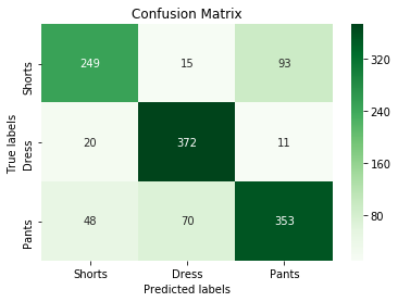
As you can see from the confusion matrix, the result looks pretty decent. Possible next moves may be to test out different network architectures, look at different labels, add more examples from other datasets, and look at using different losses and optimizers to aid in the training. The overall accuracy of the testing data was 80% so there is some room to improve, but the results are much better than the previous post.
The confusion matrix does confirm the issue with the pants and shorts as there are 93 misclassifications for pants and shorts. If feel that the majority of the classification errors may come from the data mainly as it is subjective as to what a pair of shorts are and what are short pants. To overcome this issue, a better data separation technique should be made to be more strict as to what should and should not be classified as pants and shorts.
Hazewinkel, Michiel, ed. (2001) [1994], "Binomial distribution", Encyclopedia of Mathematics, Springer Science+Business Media B.V. / Kluwer Academic Publishers, ISBN 978-1-55608-010-4