ユニファ開発者ブログ

ユニファ株式会社プロダクトデベロップメント本部メンバーによるブログです。

ユニファのエンジニア採用に興味がある人をベイズ推定で見極める

はじめに


こんにちわ、研究開発部の島田です。

先日、2019年度 人工知能学会全国大会が行われ、なんと弊社はプラチナスポンサーとして協賛し、ブースも出展させていただきました。当日は研究開発部のメンバーが総出で対応を行ったのですが、その際に色々な方から応援メッセージをいただけたので大変嬉しかったです。

学会の参加報告については、Podcastでも公開されていますのでご興味ある方はぜひこちらもどうぞ。

podcast.unifa-e.com

さて、会社としての学会参加の目的はいくつかあるわけですが、その中の一つとして”採用”があります。ですので、ブース対応するユニファ社員の関心事の一つとして、この人は「採用に興味があるのか、無いのか」になります。

採用に興味がある人であれば、出来るだけ短時間でかつ詳細に採用情報について知りたいはずです。そういう人に対しては的確な採用情報をなるべく早く与えてあげるべきですよね。

一方で、採用に興味が無い人に対して、採用情報ばかり提供してもお互いにとって良い時間の使い方にはならないはずです。

採用経験豊富な方であれば、目の前の人がどちらのタイプかをすぐに見極めるられるのでしょう。しかし、私みたいな初心者には無理です。。。それならエンジニアらしく、この直感的な判断を数値化してみよう!と思い立ちました。

ということで、前置きが長くなりましたが今回の記事は、学会のブースに来た人が採用に興味があるか否かを数値化してみたいと思います。

※ただし、本記事で計算に使う各パラメータは全て架空のパラメータとします。

ベイズ推定


さて、目的の数値化のために、今回はベイズ推定を使いたいと思います。

ベイズ推定は、一般的には下記のように説明されます。

ベイズ確率の考え方に基づき、観測事象(観測された事実)から、推定したい事柄(それの起因である原因事象)を、確率的な意味で推論することを指す。

出典:Wikipedia

小難しく聞こえますが要するに、観測されたある事実を使って推定したい事柄を確率的に求める手法のことです。 ベイズ統計学という分野は昔からありましたが、最近また注目を浴びてきました。

例えば、MicrosoftやGoogleなどでもベイズ統計の技術を活かしていることで知られています。

ベイズ統計の特徴(強み)は以下があげられます。

  • 事前知識を取り入れることで、少ないデータでもある程度の精度で推測可能。

  • 入力情報によって瞬時にそして自動的に推測を更新する

  • 逐次合理性が成り立つ

ベイズ推定の流れ


はじめに今回のベイズ推定の処理の流れについて見ていきます。

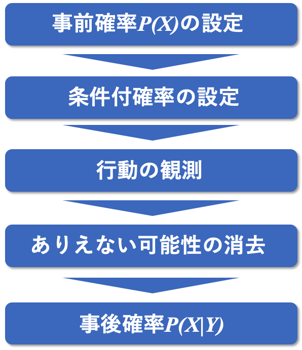
大まかにはこういう流れで進めていきます。

f:id:unifa_tech:20190624094838p:plain:w300

事前確率の設定


今回推定したいのは、ブースに来た人が採用に「興味ある」か「興味ない」かということです。そのために、推定の最初にすべきことはこの二つのタイプに対して、その割合を割り振ることです。この割合は経験に基づく設定の仕方と、そうでない割り当て方がありますが、ここでは、経験から数値が分かっているものとします。

例えば、経験的にブースを見に来た人の中で採用に「興味ある(P(A))」割合が10%(0.1)で、「興味ない(P(B))」割合が90%(0.9)だったとします。そうすると、事前確率は以下のように表せます。

P(A) = 0.1, P(B) = 0.9

条件付き確率の設定


次に、採用に興味あるかないかの二つのタイプに属する人の中で、それぞれどのくらいの割合でブースにいた弊社社員に「声をかけた」かを設定します。この条件付き確率では何らかの経験による裏付けや実験的な結果(数値)が必須です。ここでは、この結果(確率)も分かっているものとします。

例えば、「採用に興味がある人」は以下のような条件付き確率を設定します。

  • 「採用に興味がある かつ 声をかける(P(声かけ|A))」割合が80%(0.8)

  • 「採用に興味がある かつ 声をかけない(P(声なし|A))」割合が20%(0.2)

一方、「採用に興味がない人」は以下のように設定します。

  • 「採用に興味がない かつ 声をかける(P(声かけ|B))」割合が40%(0.4)

  • 「採用に興味がない かつ 声をかけない(P(声なし|B))」割合が60%(0.6)

行動の観測、ありえない可能性の消去


前項までの設定をし、実際に学会のブース対応したと仮定します。そしてありがたいことに、ある一人の方に声をかけられたとします。

これは一人の行動を実際に観測したことになり、「声かけしない」という可能性が消えて、確率が変化しました。

つまり、この実際の観測により、世界は以下の二つに限定されました。

  1. 「採用に興味ある&声かける」P(A and 声かけ)

  2. 「採用に興味ない&声かける」P(B and 声かけ)

それぞれの確率を計算します。

P(A and 声かけ) = P(A) × P(声かけ|A) = 0.1 × 0.8 = 0.08
P(B and 声かけ) = P(B) × P(声かけ|B) = 0.9 × 0.4 = 0.36

事後確率を求める


では、いよいよ本題である「声かけをしてきた人で採用に興味がある確率」P(A|声かけ)を求めます。

前項にて、観測された事実からありえない可能性を消去し世界が変化したことで、確率の和が1にならなくなりました。

そこで、それぞれの確率の組を正規化(足して1になるようにする処理のこと)を行い、事後確率P(A|声かけ)を求めます。

P(A|声かけ) = \frac{P(声かけ|A)P(A)}{P(声かけ|A)P(A)+P(声かけ|B)P(B)}
 \qquad= \frac{0.08}{0.08 + 0.36} = 0.18

この結果から、声をかけていただいた人が「採用に興味がある」確率は、約18%であると推定できました。

更に一つ大事なこととして、事前確率の設定の段階で「採用に興味がある人」と仮定したのは、10%でした。 ですが、「声をかける」という実際の事象を観測した後には、その人が採用に興味がある確率は、0.1から0.18と2倍弱にまで値が更新されました(これをベイズ更新と言います)。

このようにデータが与えられる度に値が更新されていくのもベイズ推定の一つの特徴でもあります。

おわりに


ベイズ推定を簡単に応用したケースを紹介してみましたが、いかがでしたでしょうか。

ベイズ推定は実際のビジネスシーンにおいてもかなり幅広く応用できる手法ですので、今後も色々と試してみたいと思います。

また、冒頭でもお伝えした通り、今回のブース出展では大変多くの方に応援のメッセージを頂きました!皆さんの期待を裏切らないためにも日々精進していきたいと思います。

iOSで光学的文字認識(OCR)を試してみる

こんにちは、iOSエンジニアの大江です。

最近は梅雨入りしたと言っているのに全く雨が降らず、 安心しきっています。 安心したところにいきなりくるときがあるので、みなさん油断せずいきましょう!

ということで、雨に負けないよう楽しくOCRのお話をしていきたいと思います。

前提

今回はいかにお金をかけずに手軽にやるかに重点を置いてみます!

iOSでのOCR

iOSでOCRを行うには以下のような方法があります。

ライブラリ
クラウド Google Cloud Vision API
端末 Tesseract OCR iOS
SwiftOCR
SwiftyTesseract
Firebase MLKit(β)

クラウド

Google Cloud Vision API
言わずと知れた Google さんの出しているAPIです。
一度画像をアップロードする必要があるものの、
様々なファイルタイプに対応しており、言語も自動で判別してくれます。 1ヶ月に1000ユニットまでは無料ですが、それを越えると1000ユニットごとにお金がかかります。

端末

Tesseract OCR iOS, SwiftOCR, SwiftyTesseract
それぞれオープンソースのライブラリであり、
オフラインで利用することができます!

Tesseract OCR iOS はOCRエンジンにGoogle開発のTesseractを採用しており、情報量も多くあります。
しかし、学習データのバージョンが少し古いので精度に不安が残ります。

SwiftOCR はTesseractよりパフォーマンスが良いことをアピールしています。
ただし、短い英数字を読み取るのが得意らしいので、文章などを読み込むためにはTesseractの方が良いと説明しています。
また、日本語を読み取るためには学習データを作成する必要があります。

SwiftyTesseract は Tesseract OCR iOSと同じTesseract をOCRエンジンとして採用しています。
Tesseract OCR iOS との違いとしては、最新の安定バージョンのTesseractを使用しているので、
パフォーマンスが向上しています。
ただし、Tesseract本体のAPIに完全対応しているわけではないので、利用できない機能があります。

両方

Firebase MLKit(β)

Firebase MLKit(β) はβ版ながらクラウド版と端末版両方が用意されています。
しかし、端末版ではいくつかの言語しか対応していません。
日本語はというと・・・・・・・対応していません!!
なんてこった!!
今回は日本語が試したいので、お休みしておいてもらいます。

準備

今回はSwiftyTesseractを試してみたいと思います。

  • macOS 10.14.5
  • Xcode 10.2.1 (Swift 4.2)
  • CocoaPods 1.6.2

実装

何はともあれ初めはこれです。
Xcodeプロジェクト作成しCocoaPodsをinitしてください。
やり方については、先達の方々の記事が検索すれば出てくると思うので、
そちらを参考にしていただければと思います。

SwiftyTesseractの導入

プロジェクトのPodfile を開いて以下の一行を追加します。

>pod 'SwiftyTesseract', '~> 2.0'

次にPodfileを保存して、下記のコマンドでインストールします。

$ pod install

これでSwiftyTesseractの導入は完了です! 簡単ですね!

学習データの追加

SwiftyTesseract ではTesseract用に用意されているデータを利用することができます。
Tesseract用の学習データには、次の3つのタイプが用意されています。

  • tessdata_best (LSTM、正確性重視)
  • tessdata_fast (LSTM、速度重視)
  • tessdata (パターン認識とLSTMの組み合わせ)

SwiftyTesseractによると多くの場合tessdata_fast が最良になるとのことだったので、
今回はtessdata_fast を利用します。

  1. tessdata_fastのリポジトリにアクセスし、jpn.traineddataダウンロードします。
  2. Xcodeプロジェクトにtessdataフォルダを作成ます。
  3. 作成したフォルダに、ダウンロードしてきたファイルを追加します。

これで日本語の学習データを利用する準備はできました。

画像をプロジェクトへ追加しておく

文字を読み取りたい画像ファイルを用意し、Xcodeプロジェクトへ取り込んでおきます。 今回は次の画像(sample.png)で試してみます。

f:id:unifa_tech:20190628164412p:plain
sample

この記事の一番初めの部分ですね!

OCR機能の実装

あとは実際にコードを書くだけです!
ViewController.swift で以下のように書いてあげてください。

import UIKit

// SwiftyTesseract のインポート
import SwiftyTesseract

class ViewController: UIViewController {

    // swiftyTesseract インスタンスを生成
    // この際引数で、言語の指定を行う。
    let swiftyTesseract = SwiftyTesseract(language: RecognitionLanguage.japanese)
    
    override func viewDidLoad() {
        super.viewDidLoad()

        let filename = "sample.png"
        guard let image = UIImage(named: filename) else { return }
        
        swiftyTesseract.performOCR(on: image, completionHandler: { recognizedString in
            guard let text = recognizedString else { return }
            print(text)
        })
    }
}

結果

気になる結果です!! 100%完璧とまでは行きませんでしたが、
まずまずの結果となっているのではないでしょうか。

っss 10Sで光学的文字認識(OcR)を試してみる
28
ロiOS     ロロSwift
こんにちは、iOSエンジニアの大江です。
最近は梅坪入りしたと言っているのに全く雨が降らず、 安心しきっています。 安心し
たところにいきなりくるときがあるので、みなさん油断せずいきましょう!
ということで、雨に負けないよう楽しくOCRのお話をしていきたいと思います。
前提
今回はいかにお金をかけし
たところにいきなりくるときがあるので、みなさん油断せずいきましょう!
ということで、雨に負けないよう楽しくOCRのお話をしていきたいと思います。
前提
今回はいかにお金をかけ\343\201ずに手軽にやるかに重点を置いてみます !
i0SでのOCR
i0SでOCRを行うには以下のような方法があります。
ライブラリ
クラウド Google Cloud Vision API
端末           Tesseract OCRiOS
SwiftOCR
SwiftyTesseract
Firebase MLKitB)
クラウド

まとめ

今回はタイピングされた文字を読み込みましたが、
手書きの場合はどうなるのかなど、まだ気になる箇所は残っています。
また、記事には載せていませんが、背景色によって読み取り精度ががグッと下がったので、
そこも課題かなと思いました。

しかし、個人で試して楽しむだけなら手軽にできるので、
ぜひ試してみてください!

梅雨に負けずに頑張りましょう!!

Reinforcement Learning - Q-tables

Q-Learning.

By Matthew Millar R&D Scientist at ユニファ

Q -learning is a model-free approach to reinforcement learning. This means that Q-learning does not rely on a model to make decisions based on an input, but instead uses a policy that shows the agent what actions to perform given a certain circumstance. Q-learning should find the best policy which gives an optimal solution to any finite Markov decision process. The FMDP can be described as:

f:id:unifa_tech:20190618170426g:plain
FMPD

Where X is the state space, A is the action space, and r is the reward function. The optimal solution is obtained by maximizing the total reward for any action and any change in state, starting with the current state. The best or optimal solution can be found for any finite problem given an unlimited exploration time combined with an exploration adaption to a policy. This optimal Q-function can be calculated as such:

f:id:unifa_tech:20190618170517g:plain
Q-Function

The full equation and explanation can be found in Melo’s Convergence of Q-Learning: A Simple Proof [1]:
Influences on how the agent will learn using Q-learning comes down to three real factors. Learning rate controls how much, or the rate in which new information replaces older information. If the learning rate is set to 0, then the agent will never learn anything new and will rely on previous knowledge to choose its actions. If the rate is set to 1, then the agent will only look at the most recent data and completely discard previous data.

The Discount factor is another variable that controls learning. The discount factor determines the weight of future rewards and how important or not these rewards will be. If it is set to 0, then the model will only consider instant rewards or the current reward and not look towards potential rewards of future actions. If the discount factor is set to 1, then the agent will work towards achieving the long-term highest reward.

The third and final variable used for learning the control is the initial conditions or Q0. Q-learning is an iterative program, it must have a starting condition before any changes take place to any state or environment. To help an agent explore options better, high initial values should be used regardless of which action is used. The update rules can control the values compared to other alternatives which can increase its total probability of being chosen. This will allow for each option to be fully explored and to aid in finding an optimal solution to each problem.

Q-Tables:

Q-Learning runs off a table or matrix of state and actions. This Q-table starts out all values as 0 and after each episode, these values are updated accordingly. The matrix should take the size of both the state as well as the action size with a very basic form of this is a simple array [state, action]. The simplest method for creating a Q-table in python is this:

import numpy as np
# Initial Q-table
Q_table = np.zeros((state_size, action_size))

This Q-table will store every action and state that the agent will be in. Exploitation is done when an action that has been performed before and in a certain state is chosen which results in a reward (most likely the max possible future reward). Exploration is choosing a random action at any point in time and in any state. A basic method for this could be defined as below:

import random
epli = 0.4
def choose_action (epli)::
	ran_float = random.random() # Generates a random float between [0,1]
	if ran_float < epli:
		#preform a random action
	else:
		get_action_from_qtable(current_state, q_table)

After choosing an action to perform and receiving a reward, the Q-table must be updated. The updating must be done after each action is performed. The updating phase will end at the conclusion of each episode. The basic flow of the update function will be:

Step 1: Get the current state of the agent.
Step 2: The agent takes action. (Picks random action or Pick action from Q-table)
Step 3: Update q-value.
An update rule for Q-values can be described as:

Q[state, action] = Q[state, action] + learning_rate * (reward + gamma * np.max(Q[new_state, :])) – Q[state, action] 

This is a basic approach to adjust and update q-values in a Q-table.

Now for a simple example:
First lest look at the agent in the game:

class Agent:
    def __init__(self, learning_rate = 0.1,
                discount = 0.95,
                 exploration_rate = 1.0,
                iterations = 1000):
        # Q talbe for holding rewards
        self.q_table = [[0,0,0,0,0], [0,0,0,0,0]]
        self.learning_rate = learning_rate
        self.discount = discount # Future rewards value to current rewards
        self.exploration_rate = exploration_rate # Exploration rate
        # This controls sift from exploration to exploation
        self.exploration_delta = 1.0 / iterations
        
    # Chose between explotation or exploration
    def get_next_action(self, state):
        if random.random() > self.exploration_rate:
            return self.greedy_action(state)
        else:
            return self.random_action()
    
    def greedy_action(self, state):
        # Check to see if forward is best reward
        if self.q_table[FORWARD][state] > self.q_table[BACKWARD][state]:
            return FORWARD
        elif self.q_table[BACKWARD][state] > self.q_table[FORWARD][state]:
            return BACKWARD
         # Rewards are equal, take random action
        return FORWARD if random.random() < 0.5 else BACKWARD
    
    def random_action(self):
        return FORWARD if random.random() < 0.5 else BACKWARD
    
    def update(self, old_state, new_state, action, reward):
        old_value = self.q_table[action][old_state]
        # best next action 
        future_action = self.greedy_action(new_state)
        # reward for the best next action
        future_reward = self.q_table[future_action][new_state]

        # Main Q-table updating algorithm
        new_value = old_value + self.learning_rate * (reward + self.discount * future_reward - old_value)
        self.q_table[action][old_state] = new_value

        # Finally shift our exploration_rate toward zero (less gambling)
        if self.exploration_rate > 0:
            self.exploration_rate -= self.exploration_delta

Then lets built the environment that he can walk through.

# Build the Environment
class EnvironmentSimulator:
    def __init__(self, length=5, small=2, large=10):
        self.length = length # Length of the environment 
        self.small = small  # reward for going back to the start
        self.large = large  # reward for reaching the end
        self.state = 0  # environment entry point

    def take_action(self, action):
        if action == BACKWARD:  
            reward = self.small
            self.state = 0
        elif action == FORWARD: 
            if self.state < self.length - 1:
                self.state += 1
                reward = 0
            else:
                reward = self.large
        return self.state, reward
    # Reset the environment
    def reset(self):
        self.state = 0  
        return self.state


This is a very simple array of 5 spaces. So basically, the agent can walk back a forth and get a reward for either reaching one end or the other.
Next, we will set up the environment and the main loop for running the simulation.

# Set up environment
environment = EnvironmentSimulator()
environment.reset()
# Scores
total_reward = 0
last_total = 0

for step in range(iterations):
    # Store the current state in old state
    old_state = environment.state
    action = agent.get_next_action(old_state)
    new_state, reward = environment.take_action(action)
    agent.update(old_state, new_state, action, reward)
    
    total_reward += reward
    if step % 250 ==0:
        performance = (total_reward - last_total) / 250.0
        print("Step:{} Performance:{} Total-reward:{}".format(step, performance, total_reward))

RI Hello World Revisited

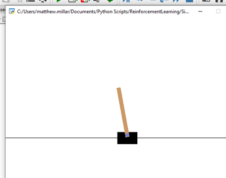
Let's take a look back at the Cart Pole example from the previous blog,
tech.unifa-e.com
We did that with a Keras model, now we will do it with a q-table approach.

First we need to set up the Q-learning class

class QLearn:
    def __init__(self, actions, epsilon, alpha, gamma):
        self.q = {}
        self.epsilon = epsilon  
        self.alpha = alpha      
        self.gamma = gamma      
        self.actions = actions

Next, we need a few methods for choosing actions and updating the tables:

    # Q learning function
    def learnQ(self, state, action, reward, value):
        old_value = self.q.get((state, action), None)
        # If there are no values in the table add the reward
        if old_value is None:
            self.q[(state, action)] = reward
        else:
            self.q[(state, action)] = old_value + self.alpha * (value - old_value)

    def chooseAction(self, state):
        q = [self.getQ(state, a) for a in self.actions]
        maxQ = max(q)

        if random.random() < self.epsilon:
            minQ = min(q); mag = max(abs(minQ), abs(maxQ))
            q = [q[i] + random.random() * mag - .5 * mag for i in range(len(self.actions))] 
            maxQ = max(q)

        count = q.count(maxQ)
        if count > 1:
            best = [i for i in range(len(self.actions)) if q[i] == maxQ]
            i = random.choice(best)
        else:
            i = q.index(maxQ)
        action = self.actions[i]        
        return action, q

    def learn(self, s1, action, reward, s2):
        maxqnew = max([self.getQ(s2, a) for a in self.actions])
        self.learnQ(s1, action, reward, reward + self.gamma*maxqnew)

And now let's define the main method:

if __name__ == '__main__':
    # Load the cart pole game from gym ai
    env = gym.make('CartPole-v0')
    # Vriables needed
    max_number_of_steps = 200
    last_time_steps = numpy.ndarray(0)
    n_bins = 8
    n_bins_angle = 10
    max_number_episodes = 200
    episode_number = 0
    render = False

    number_of_features = env.observation_space.shape[0]
    last_time_steps = numpy.ndarray(0)

    # Simplfy the number of states as it is too large
    cart_position = pandas.cut([-2.4, 2.4], bins=n_bins, retbins=True)[1][1:-1]
    pole_angle = pandas.cut([-2, 2], bins=n_bins_angle, retbins=True)[1][1:-1]
    cart_velocity = pandas.cut([-1, 1], bins=n_bins, retbins=True)[1][1:-1]
    angle_rate = pandas.cut([-3.5, 3.5], bins=n_bins_angle, retbins=True)[1][1:-1]


    qlearn = QLearn(actions=range(env.action_space.n),
                    alpha=0.5, gamma=0.90, epsilon=0.1)

    while episode_number < max_number_episodes:
        observation = env.reset()

        cart_position, pole_angle, cart_velocity, angle_rate_of_change = observation
        state = build_state([to_bin(cart_position, cart_position),
                         to_bin(pole_angle, pole_angle),
                         to_bin(cart_velocity, cart_velocity),
                         to_bin(angle_rate_of_change, angle_rate)])

        for t in range(0, max_number_of_steps):
            if render:
                env.render()

            action = qlearn.chooseAction(state)
            observation, reward, done, info = env.step(action)

            cart_position, pole_angle, cart_velocity, angle_rate_of_change = observation
            nextState = build_state([to_bin(cart_position, cart_position),
                             to_bin(pole_angle, pole_angle),
                             to_bin(cart_velocity, cart_velocity),
                             to_bin(angle_rate_of_change, angle_rate)])

            if not(done):
                qlearn.learn(state, action, reward, nextState)
                state = nextState
            else:
                # Penalize it for failing
                reward = -200
                qlearn.learn(state, action, reward, nextState)
                last_time_steps = numpy.append(last_time_steps, [int(t + 1)])
                break

And that is really the only difference between the Keras and q-learning ways of solving the Cart Pole problem.
Instead of the model deciding what to do, the values in the q-table are making the decision.

Conclusion

This shows how to simply set up an environment and use a q-table to learn RI. This was a simple example the next logical step would be to have a negative reward which would encourage the AI to stop moving backward and to only move forward. This could help shape how the AI will learn and help move it towards the desired actions. This program is really a bare-bones approach with no bells and whistles. It shows you what is the minimum to have for an agent, environment, and simulation for training up a RI agent.
We also revisited the cart pole example to see how Q-Learning can be done compared to using a Keras model. The Keras model needs less code and can solve the issue a little better than the Q-learning approach. This may be because I had to simplify the states that the pole can take which may lead to the poorer results.
Q-learning has its limits as the table can become very complex as the states and actions that are a possible increase in the total number. This can greatly increase the complexity of the Q-table which can become very difficult to manage. By simplifying the dimensions of the state/action sets can help make it more manageable, but you sacrifice granularity which can lead to mistakes in the results.

Resources:

[1]: Melo, F. Convergence of Q-learning: a simple proof. Retrieved 2019 from

JSAI2019に参加してきました

はじめまして。R&Dチームの宮崎です。 普段はルクミーフォトを よりスマートにすべく画像認識の研究開発に取り組んでいます。 今回はユニファのR&DチームでJSAI2019に参加してきたので、その様子を報告をしたいと思います。

また、JSAI2019の様子はPodcastでも公開しておりますので、ご興味ある方はあわせて聴いていただければと思います。

12. AIにとっての「正しさ」って何なんだろう | UniFa Developer's Podcast

続きを読む

シフトスケジューリング問題 (入門)

研究開発部の浅野です。普段は画像やヘルスケアデータを扱うことが多いのですが、最近シフトスケジューリング問題に興味をもって学び始めたので、その内容を少しご紹介したいと思います。シフトスケジューリング問題とは、人員の配置基準や働く人の希望、能力、相性、業務負荷などを加味しながらある一定期間(1ヶ月など)の勤務シフト表を作成する問題です。看護師のナーススケジューリングが有名ですが、保育士のシフト作成も多くの園長先生が頭を悩ませていることの一つです。今回はこの問題を最適化問題としてモデル化・定式化して実際に解いてみたいと思います。

最適化問題は、制約条件を満たす解の中で、目的関数を最小(最大)にする解を求めるもので、次のように定義されます。

\begin{align} minimize \quad &f(x): &目的関数\\ subject \; to \\ &g(x)>= 0: &不等式制約条件\\ &h(x) = 0: &等式制約条件\\ &a <= x <= b: &変数\\ \end{align}

我が家のシフトスケジューリング問題

共働きで3人の子どもを育てており、朝の支度と夜のお迎えから寝かしつけまでを夫婦どちらが担当するのか、仕事などの都合を考慮して決めています。週の終わりにお互いの来週の予定を共有し、それをもとに1週間分のシフトを作成します。それぞれの都合を尊重しつつ公平性を保った配分を手作業で決めるのは結構面倒です。

それではこの問題を徐々にモデル化および定式化していきましょう。メンバー mが曜日 dにアクション aを担当するときに 1、そうでないときに 0となる変数 x_{mda}を使います。夫婦がどちらも都合が悪い場合に奥様の母上がヘルプに入ってくれてとても助かっているのですが、それに甘えすぎると大切な子どもとの時間を仕事などに割り振ってしまう傾向が強まります。そこで目的関数として母上のヘルプ回数を設定し、それを最小化するという問題設定にします。

 \displaystyle
minimize  \sum_{d \in D, \, a \in A} x_{母da} \qquad D=\{Mon, Tue, Wed, Thu, Fri\}, \, A=\{朝, お迎え\}

これは我が家ではこうするのがよい、ということであり、各家庭の状況によって問題設定は変わります。このように、どんな目的関数を設定してどのような制約条件を設けるかというモデリングはかなりドメインの知識を必要とする作業です。

それではここまでの部分をコードに落としてみましょう。PythonのPuLPという最適化問題のモデリングを簡単にコーディングできるライブラリを用います。PuLPには汎用ソルバーもバンドルされているため、そのまま解を求めることも可能です。

import pulp

Member = ["夫", "妻", "母"] 
Day = ["Mon", "Tue", "Wed", "Thu", "Fri"] 
Action = ["朝", "お迎え"] 

#問題の宣言
ShiftScheduling = pulp.LpProblem("ShiftScheduling", pulp.LpMinimize)

#変数宣言
x = {}
for m in Member:
    for d in Day:
        for a in Action:
            x[m, d, a] = pulp.LpVariable("x({:},{:},{:})".format(m,d,a), 0, 1, pulp.LpInteger)

#目的関数:母からのヘルプを最小限に抑える
ShiftScheduling += pulp.lpSum(x['母', d, a] for d in Day for a in Action), "Target"

制約条件

制約条件として、まず下記を考えます。

 \displaystyle  \sum_{m \in M} x_{mda}=1 \qquad M=\{夫、妻、母\}, \, d \in D, \, a \in A

これは毎日朝とお迎えには誰か1人が必ずアサインされる、という意味です。そうしないと子ども達が路頭に迷ってしまいます。次に、この日は朝早く出社したい、あるいは遅くなるからお迎えに行けない、といった条件を加えます。

 \displaystyle   x_{mda}=0 \qquad (m,d,a) \in NG, \quad NG=\{(m, d, a) | メンバーmは曜日dにアクションaが不可能\}

これらをコードにすると下記のようになります。夫は火曜朝と木曜夜、妻は水曜夜、(宿泊出張で)木曜夜と金曜の朝が都合が悪い(実際よくあるパターン)、としています。

# それぞれの日の朝やお迎えに必ず誰か1人が割り当てられる
for d in Day:
    for a in Action:
        ShiftScheduling += pulp.lpSum(x[m, d, a] for m in Member) == 1, "Constraint_{:}_{:}".format(d,a)

# 対応不可能日
NG = [['夫','Tue','朝'],['妻','Wed','お迎え'],['夫','Thu','お迎え'],['妻','Thu','お迎え'],['妻','Fri','朝']]
for m, d, a in NG:
    ShiftScheduling += x[m, d, a] == 0, "Constraint_NG_{:}_{:}_{:}".format(m,d,a)

解いてみる

では一旦この状態で最適化問題を解いてみましょう。 solve()関数を呼ぶだけです。その結果作成されたシフトも示します。

results = ShiftScheduling.solve()
print("optimality = {:}, target value = {:}".format(pulp.LpStatus[results], pulp.value(ShiftScheduling.objective)))

 optimality = Optimal, \quad target \, value = 1.0

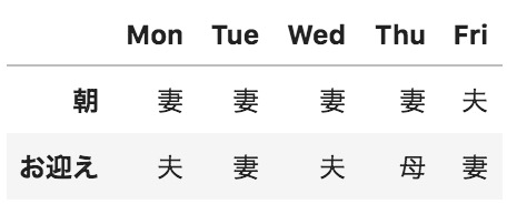
f:id:unifa_tech:20190616233256j:plain:w300
自動で計算されたシフト

print文の出力は、最適解が見つかったことと、母上の出動が1回あることを示しています。確かに木曜のお迎えは夫婦どちらも対応できないのでやむを得ません。他の都合が悪い日についてもちゃんと考慮されたシフトになっています。ただしこれをこのまま奥様に見せたら不公平だとお怒りになりますね。

制約条件の追加

そこで1週間の出動回数の差が大きくならないように制約条件を追加します。数式は割愛してコードと結果を示します。

# 週全体で出動回数の差を抑える
n_act_wife = pulp.lpSum(x['妻', d, a] for d in Day for a in Action)
n_act_husband = pulp.lpSum(x['夫',d, a] for d in Day for a in Action)
ShiftScheduling += n_act_wife - n_act_husband <= 1, "Constraint_fairness_wife"
ShiftScheduling += n_act_husband - n_act_wife <= 1, "Constraint_fairness_husband"

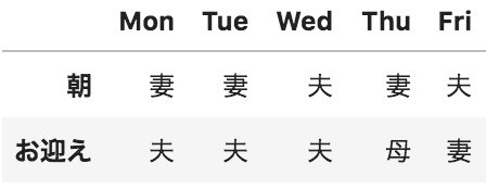
f:id:unifa_tech:20190616234538j:plain:w300
出動回数を調整したシフト

これで奥様の怒りも収まりますね。しかしよく見ると水曜日は朝もお迎えも自分が担当になっていて、できなくはないのですがちと辛い。そこでもう一つ制約条件を加えて朝とお迎えが重ならないようにします。ここも数式は割愛。

# 1日で朝かお迎えどちらかだけ
for m in Member:
    for d in Day:
        ShiftScheduling += pulp.lpSum(x[m, d, a] for a in Action) <= 1, "Constraint_Either_{:}_{:}".format(m,d)

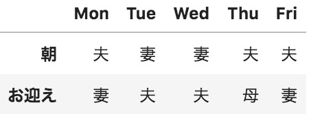
f:id:unifa_tech:20190616235159j:plain:w300
朝とお迎えが重ならないようにしたシフト

いいシフトができました。今後は都合の悪い日をインプットするだけで自動的に公平な分担表を作成できて楽になります。

まとめ

シフトスケジューリング問題に対して、最適化問題としてのモデル化、定式化、コードへの実装を一通り行うことができました。今回扱ったのは登場メンバーが3人で1週間分の朝とお迎えシフトを決めるという比較的小さな問題で、変数の数が30しかないため解は一瞬で得られます。実際の保育士のシフト作成は、数十人の保育士さんの1ヶ月分の勤務(早番、中番、遅番など)を、園児の人数あたりの保育士配置基準、ベテランと若手のミックス、研修や休暇などの予定、シフトに入れる時間帯の制約、体調などを考慮に入れて作成します。変数の数や制約条件が桁違いに多くなるため複雑な作業になりますが、ドメイン知識を使ってモデル化し、目的関数や制約条件をうまく定式化し、ソルバーを使って解くという流れは同じです。こうした技術を使って保育園での作業負担をどんどん減らしていきたいですね。

AI Stock Price Prediction Methods.

By Matthew Millar R&D Scientist at ユニファ

Summary:

            This blog is looking at finding the best method for future price prediction for stocks in general.  This blog will look at methods for calculating production that is in current research and uses in the industry.  Also, it will cover; statistical methods, machine learning, artificial neural networks, and hybrid models.  From the current research, hybrid models were found to give the best results over pure statistical methods and pure machine learning and artificial neural network methodologies.

Introduction:

            Stock market prediction is a method to discover possible future values of a stock.  With successful predictions of prices, higher profits can be gained, but on the other hand with bad predictions can produce losses.  There is a standard thought that the market does not follow a standard flow, so predictions using statistics or models would be an impossible task due to the idea that technical factors cannot show all of the variables that help shape the movement of the stock market.  On the contrary, the efficient market hypothesis would otherwise suggest, a stock price already reflects all the information that could affect any price changes except for unknown information which is always a level of unpredictability.

            Fundamental analysis looks at the company rather than just the numbers or charts.  This involves looking at the past performance and credibility of its accounts.  This approach is mainly used by fund managers as this is one of the traditional methods that use publicly available information on the company.  Technical analysis does not care about the company's fundamentals but mainly look at the trends of the stocks past performance in a time series analysis.  These are the two more common ways of stock price prediction.  Current trends in price forecasting are the use of Data mining technologies.  The use of Artificial Neural Networks (ANN), Machine Learning (ML) algorithms, and statistical models are now being used to help in prediction.       

            Due to the increasing amount of data from trades, data mining and data analysis on this amount of data can be very difficult using standard methods.  With the amount of data that is produced daily, this could be considered on the level of Big Data analytics.  Due to the ever-changing values of the data throughout the day, it is difficult to monitor every stock that is available, let alone to perform prediction on price movements.  This is where the use of algorithms and models come into play.  With these algorithmic models, predictions can be made with relative accuracy and can give investors better insight into the actual data's value without all of the excessive amounts of data review.

Goal:

            The goal of this blog is to look at possible methods for prediction using ML, ANN, and statistical models.  Statistical methods are the most commonly used method for price prediction currently, but will the use of ML, ANN, or hybrid systems can give a more accurate prediction. It will continue to look at statistical methods, pure ML, pure ANN, and hybrid models, a more comprehensive list can be made, and a better idea of which approach could be better for forecasting purposes.   

Methodology Review:

            There are a few emerging methods that are gaining popularity and applications over the traditional financial approaches.  These methods are based on ML, statistical models, ANN, or a hybrid model.  Some of the proposed models use a purely statistical method, some use pure ML or ANN, and others use a hybrid approach combining both statistical and ML or ANN together.  Each model has its pros and cons for use and a problem that solves best.

Statistical Methods:

            By using data analysis, one can predict the closing price of a certain stock.  Currently, there are six common methods or data analysis to make a predictive model.  Some of these models are common Stock price models that are used currently in the stock market and by fund managers.  These five models are must be in agreement of the movement direction in order for the price movement to be predicted most accurately.  These models are; Typical Price (TP), Chaikin Money Flow Indicator (CMI), Stochastic Momentum Index (SMI),

Relative Strength Index (RSI), Bollinger Bands (BB), Moving Average(MA), and Bollinger Signal.  By combining these algorithms, a more accurate prediction can be made by looking at upper and lower bands, if the price goes above the upper band then that indicates a positive selling point and if it goes below the lower band it indicates a positive buy point.  This method of combining the results of other models does give a better chance of price change than just one of the single statistical models (Kannan, Sekar, Sathik, & Arumugam, 2010).

Machine Learning Artificial Neural Network Methods:            

            Text mining has also been used in stock prices trends, especially for inter day prices trends.  By using text mining techniques, a 46% chance of knowing if a stock will increase or decrease by 0.5% or remain in the positive and negative range, which was more significant than a random predictor which only gave around 33% accuracy for stock price fluctuation prediction.  By using a process of text mining, by gathering press releases and preprocess them into usable data and categorizing them into different news types.  Trading rules can then be derived from this data for particular stocks (Mittermayer, 2004).

            Pure ANN is used currently for stock prediction as well as analysis.  The users have given very reliable results as ANN are good at working with errors, can use large and complex data, and can produce useful prediction results.  For forecasting just one stock, there is a lot of interacting input series that is needed.  Each neuron can represent a decision process.  This will allow for ANN to represent the interaction between the decisions of everyone in the market.  This will allow for the ANN to completely model a market.  ANN is very effective at predicting stock prices (Kimoto, Asakawa, Yoda, & Takeoka, 1990; Li, & Ma, 2010),

            ANN is gaining acceptance in the financial sector.  There are many techniques and application that look into using AI in creating prediction models.  One common method is to use a genetic algorithm (GA) to aid in the training or the ANN for the prediction of stock prices.  The GA, in most cases, are used for training the network, selecting the feature subset, and aiding in topology optimization.  A GA can be used to help in the feature discretionary and determination of connection weights for an ANN (Kim and Ham, 2000).

Hybrid Models:

            ML combined with an AI is a very good combination of two very powerful methodologies.  An ML model can be used for data mining to define and predict the relationships between both financial and economic variables.  The examination of the level estimation and classification can be used for a prediction of future values.  Multiple studies show that by using a classification model, a trading strategy can generate higher risk-adjusted profits than the traditional buy and hold strategy as well as the level estimation prediction capability of an ANN or linear regression (Enke and Thawornwong, 2005).  ML is mainly based on supervised learning which is not appropriate for long term goals.  But, by using reinforcement learning ML, is more suitable for modeling real-world situations much like stock price prediction.  By looking at stock price prediction as a Markov process, ML with the TD(0) reinforcement learning algorithm that focuses on learning from experiences which are combined with an ANN is taught the states of each stock price trend at given times.  There is an issue with this in that if the prediction period is either very short or very long, the accuracy decays drastically.  So this would only be useful for mid-range prediction for prices (Lee, 2001).  Another Hybrid model that has given great accuracy (around 77%) is combining a decision tree and an ANN together.  By using the decision tree to create the rules for the forecasting decision and the ANN to generate the prediction.  This combination is more accurate than either an ANN or a decision tree separately (Tsai and Wang, 2009).

Other Useful Models:

            Support Vector Machines have also been used for stock market prediction.  SVM does perform better than random guessing but are out shown by hybrid models.  A combination of a genetic algorithm and an SVM can produce a better result than even an SVM alone.  By using some technical analysis fields used as input features.  This method was used to not only produce a forecast for the stock that is being looked at as well as any other stock that has a correlation between each other and the target stock.  This hybrid significantly can outperform a standalone SVM (Choudhry and Garg, 2008). 

Discussion:

            There are many ways to produce a future value prediction, though some are slightly better and more accurate than others.  Statistical analysis is the most common approach to prediction.  Linear regression, logistic regression, time series models, etc... are some of the more common ways of predicting future values.  But, these methods may not be the best for more complex and dynamic data sets.  If the data is not the same type, linear regression may have poor results.  This is where an ANN or ML model comes in.  These can produce a better result which a higher accuracy than a purely statistical approach as they can work with the complex systems of a market.  In the pure form, an ANN or ML can produce better accuracy over many statistical methods for most stock price predictions.  But, by using hybrid ANN, an even more accurate and useful model can be done.  By combining a DT or a GA with an ANN, a greater accuracy over the two pure methods can be gained.   


Reference:

Choudhry, R., & Garg, K. (2008). A Hybrid Machine Learning System for Stock Market Forecasting. World Academy of Science, Engineering and Technology International Journal of Computer and Information Engineering, 2(3).


Enke, D., & Thawornwong, S. (2005). The use of data mining and neural networks for forecasting stock market returns. Expert Systems with Applications, 29(4), 927-940.


Kannan, K., Sekar, P., Sathik, M., & Arumugam, P. (2010). Financial Stock Market Forecast using Data Mining Techniques. Proceedings of the International MultiConferences of Engineers and Computer Scientists, 1.


Kim, K., & Han, I. (2000). Genetic algorithms approach to feature discretization in artificial neural networks for the prediction of stock price index. Expert Systems with Applications, 19(2), 125-132.


Kimoto, T., Asakawa, K., Yoda, M., & Takeoka, M. (1990). Stock market prediction system with modular neural networks. 1990 IJCNN International Joint Conference on Neural Networks.


Lee, J. W. (2001). Stock price prediction using reinforcement learning. ISIE 2001. 2001 IEEE International Symposium on Industrial Electronics Proceedings (Cat. No.01TH8570). 


Lin, Tom C. W., The New Investor. 60 UCLA Law Review 678 (2013); 60 UCLA Law Review 678 (2013); Temple University Legal Studies Research Paper No. 2013-45. Available at SSRN: https://ssrn.com/abstract=2227498


Li, Y., & Ma, W. (2010)Applications of Artificial Neural Networks in Financial Economics: A Survey. 2010 International Symposium on Computational Intelligence and Design, Computational Intelligence and Design (ISCID), 2010 International Symposium on, 211. 


Mittermayer, M. (2004). Forecasting Intraday Stock Price Trends with Text Mining Techniques. E Proceedings of the Hawai'i International Conference on System Sciences, January 5 – 8, 2004, Big Island, Hawaii.


Tsai, C. Wang, S. (2009). Stock Price Forecasting by Hybrid Machine Learning Techniques. Proceedings of the International MultiConference of Engineers and Computer Scientist 2009 Vol1 IMECS 2009. Vol 1
Reinforcement Learning the Hello World Version

By Matthew Millar R&D Scientist at ユニファ

What is Reinforcement Learning?

Reinforcement learning (RI) is a subset of Artificial Intelligence (AI) that is an agent-based approach in the field of AI. Agent-based AI learns from interacting with their environment rather than a dataset. The environment is controlled or altered by the actions of the agent. The environment changes should have goals linked to them so that the agent knows the results of each action. From this goal, appropriate actions can be learned for many different types of tasks. RI is one of the three learning techniques in machine learning. The other two are supervised and unsupervised learning. RI does not require labeled data as in supervised or semi-supervised learning.

In general, RI is a Markov Decision Process (MDP) which takes both the environment and agent states denoted a  S. It then lists out a set of all possible actions available to an agent denoted as A. There is a probability equation that shows the likely hood of transitions between states   (s1 -> s2) when a certain action  (a) is performed. The requirement of a reward is also needed to drive the system forward to learn. The normal use is an immediate reward after the transition between states denoted as  Ra(s, sl). There also must be a set of rules that control what the agent receives as feedback, or what it can observe.

f:id:unifa_tech:20190617091506g:plain
Probability

The interaction between an agent and its environment happens in discrete time steps. Each time t step will have an observation (ot ) and a reward (rt), The agent will then chose an action from its predefined set of actions (at). This action is then sent into the environment which will move the environment to its next state (st+1). As the environment moves to its next state, a new reward is then generated (rt+1). This state change can then create a transition (st, at, st+1) which allows for the agent to learn from its actions.

The agent will have to learn what is optimal behavior which leads to teaching it to regret its actions. Regret compares the performance of the current agent to that of an “optimal” agent and looks at the differences between both the actions and the awarded rewards. This is where instant rewards can hinder the performance of a model. The Agent will have to consider the long-term outcomes of its actions. This means even if the instant rewards for a certain action may be negative, the total long-term rewards could be higher. This is all to maximize future outcomes and rewards. This allows for RI to be applied to both short term goals as well as long term solutions, but not at the same time normally.

For an agent to increase the total rewards for a task, a balance between exploration and exploitation needs to be considered. Exploitation is basically using what works. This means that the agent will continue to perform actions that give it the best rewards but may not be optimal or can max out the rewards for a given set of actions. This is where exploration comes in to manage this and to hopefully optimize the result by trying different actions at any given time step. In general, simple exploration models are preferred as there are very few exploration algorithms that can scale up with a very complex environment and action sets. One way is to choose the best long-term action and then randomly choose an action at different times to see if these actions can improve on the already defined “optimal” long-term option.

There are many options to control the learning process for RI agents. The idea of how to define what actions a beneficial is still difficult to deal with correctly. The simplest method if the action set is finite is to use a policy. A policy maps the probability of action to a certain change in the state of the environment. These policies are the base of all other learning algorithms. The state-value function uses the policies by looking at the expected return of each action from the initial state and successfully follow the policy. This method evaluates the benefit of being in certain states over others. Monte Cario (MC) method can be used to mimic a policy evaluation and improvement. MC evaluation step looks at every state and action pair and averages all the returns from each state and action pair. This can compute a very accurate Q-table which can fully evaluate the policy. The improvement step uses a greedy policy and looks at each state-action pair and then computes an action that will maximize the return for each state. These are just two methods to control the learning of an RI agent.

Simple Example:

This was a very quick overview of the main principles of RI. Now let’s get to our first project.
So, let’s start with the hello world of OpenAI Gym. Note that this is just a first step on our way to the final project that I have planned.
The first step is to get all the dependencies.

Tensorflow: pip install --upgrade tensorflow
Keras: pip install Keras
Numpy: pip install numpy
OpenAI Gym: pip install gym.

Now that we have all the requirements lets get down to the nuts and bolts.
Let’s define our rewards method

Calculate Rewards (reward, gamma value)
		The new reward is reward + (previous reward * gamma value) 

This method lets us calculate the reward for every action.
Now let use a custom log loss function as well

Custom Loss (True Value, Predicted Value)
		Log(True * (true – Predicted) + (1 – ture) * (true + predicted)
		Take the mean of the results of this

Now a scoring function to see how accurate out AI is for testing.

Evaluate Model (Model, number of tests)
		Model score = 0
		Total reward = [] # Holds all rewards for each iteration
		For each iteration or run though the environment
			Sum of rewards
			Have the agent run though the environment collecting rewards
			Add the collected rewards to the Sum of rewards
			After the iteration add the final rewards 
		After each run through to add the final rewards to the total reward list
		Then you can find the mean, median, or the mode score or any other method you want

Now the keras model part

# Set up Keras model
action_count = env.action_space.n
input_shape = layers.Input(shape=env.reset().shape)
adv = layers.Input(shape=[1])

x = layers.Dense(8,activation="relu",
                 kernel_initializer=glorot_uniform(seed=42))(input_shape)
out = layers.Dense(action_count,activation="softmax",
                   kernel_initializer=glorot_uniform(seed=42))(x)

# Crate the training model and prediction model
train_model = Model(inputs=[input_shape, adv], outputs=out)
train_model.compile(loss=my_ri_loss, optimizer=Adam(lr))
test_model = Model(inputs=[input_shape], outputs=out)

This will allow us to then try out the test environment that is in OpenAI gym.
Let us start with

env = gym.make("CartPole-v0")

Putting it all together should give you this.

f:id:unifa_tech:20190614170044p:plain
CartRI
With the output of

Average reward for training episode 100: 19.30 Test Score: 13.60 Loss: 0.030333 
Average reward for training episode 200: 22.45 Test Score: 10.50 Loss: 0.022194 
…..
The average reward for training episode 8200: 25.68 Test Score: 191.40 Loss: -0.003017 
Solved in 8199 episodes!

Conclusion:

This is the end of this necessary explanation of RI. We learned the basics of reinforcement learning and how to code this up using a simple example in python. Now we can start to get into more complex models and even latter teach something to run!

Part two so soon!?!?

Well yes as this was a simple version and easy to follow. Let’s look at using a retro game and start playing stuff like Space Invaders and Mario!
The first thing we need to do is install Game-Retro using
pip3 install gym-retro
And that’s it, so to test this out we will use the built in rom from Airstriker-Genesis, but other roms can be downloaded and used here as well.

import retro
def main():
    env = retro.make(game='Airstriker-Genesis')
    obs = env.reset()
    while True:
        obs, rew, done, info = env.step(env.action_space.sample())
        env.render()
        if done:
            obs = env.reset()
    env.close()
if __name__ == "__main__":
    main()

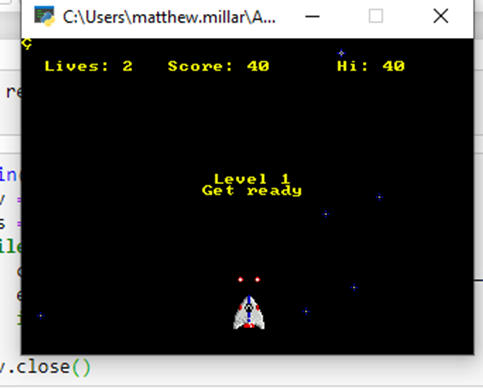
And that will give you the below screen output.

f:id:unifa_tech:20190614170236p:plain
ShooterRI

Now that we know that it is working, we need to import other games into the environment. The simplest way is to import all the ROMS that came with Gym-Retro by going into the terminal and typing this

python3 -m retro.import /path/to/your/ROMs/directory/

But you will need to find ROMs that work with gym-retro.

So our next steps that we will go after is to start with Unity3D and see how to implement RI in a 3D environment over these simpler 2D games. Soon we will look at teaching an AI to walk in the future.