MAG part II

By Matthew Millar R&D Scientist at ユニファ

Purpose:

This is part II of the MAG (Multi-Model Attribute Generator) paper I am working on. You can see part 1 here
Multi-Model Attribute Generator - ユニファ開発者ブログ
This post will focus on defining what clothing the lower half of a person is wearing. This will not look at color right now as that will follow in the next few posts. This model will allow for the classification of three different clothing types; skirts/dresses, shorts, and pants.

Processing Images:

So, from my previous post, I was only getting around 56% accuracy which is ok but not good enough. I altered my code to use a fine turned Xception model trained on the Market1501 dataset. I then used this as the base feature extractor which gave very good results in Keras. My experiments showed that the Resent50 did not produce as good results compared to Xception pre-trained models for this dataset. The data argumentation consists of rotation, cropping, vertical and horizontal shifts, and horizontal flipping. I also added a preprocessing script into the data augmentation which processes each image using the Xception preprocessing input which greatly helps in the accuracy of the model as well as keeping the handling of input consistent between this model and the base model as the Xception preprocessing was performed there as well. This aids in keeping the handling of input consistent between models and limits errors that could occur due to inconsistent preprocessing.

Clothing Makes the Man:

The first step is to separate the images into their classes for Keras to use in the data generator. This will consist of three classes, Dress/skirts, shorts, and pants.
The next step is to create the base feature extractor by importing the pre-trained model and creating a new base model using Keras Function API.

base_model = load_model('pre_trained_model.ckpt')
base_extractor = Model(inputs=base_model.input, outputs=base_model.get_layer('glb_avg_pool').output)
for layer in base_extractor.layers:
    layer.trainable = True

Note the output should be the last layer before the Softmax Fully connected layer. This will give you a feature vector over a prediction.
This will prime the base model to be used for the feature extractor. Remember you want to set each layer to trainable to allow for the base model to be retrained for the specific task. The next step is to actually build out the new model for classification.

def build():
    img = Input(shape=(224,224,3))
    # Get the base of the image
    x = base_extractor(img)    
    x = Dense(2048, activation='relu')(x)
    x = Dropout(0.2)(x)
    x = Dense(2048, activation='relu')(x)
    x = Dropout(0.2)(x)
    x = BatchNormalization()(x)
    print(x.shape)
    pred = Dense(3, activation='sigmoid')(x)
    return Model(inputs = img, outputs = pred)

Seeing that we are only looking at the lower portion of the body we will need to crop the image using a custom image generator.

# Custom cropping method for preprocessing
def crop_lower_part(img):
    # xception preprocessing an image should be called in the datagen not here in the prefrocess function
    y,x,_ = img.shape
    startx = 0
    starty = y//2
    return img[starty:y,startx:startx+x]

def crop_generator(batches):
    while True:
        batch_x, batch_y = next(batches)
        batch_crops = np.zeros((batch_x.shape[0], 112, 224, 3))
        for i in range(batch_x.shape[0]):
            batch_crops[i] = crop_lower_part(batch_x[i])
        yield (batch_crops, batch_y)

This basically cuts the image in half (the lower portion only) and create new images and send the batch to the model when needed.

Binary over Categorical loss:

We will be using binary cross-entropy over the categorical version for multi-label classification. This can be confusing as most every other model out there uses a categorical version. However, this works by treating each output label as an independent Bernoulli distribution which gives greater accuracy over the traditional approach (Hazewinkel, 2001). This will allow for each output node to be singularly penalized for the wrong answer. Which should in return give better more accurate results overall.
While categorical_crossentropy was getting 75% was decent results, by using binary_crossentropy over categorical_crossentropy, the accuracy increased by 5%.

binary_crossentropy Accuracy

binary_crossentropy Loss

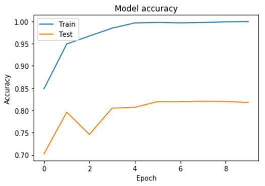
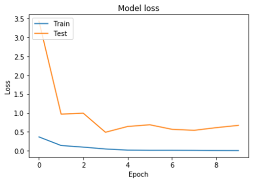
We are still overfitting after the 5 epoch, but this might be managed by cleaning the dataset by adding more samples as well as making a clear definition between shorts and pants as some samples of shorts look very close to pants. For example, some men's shorts are very long and some women's pants are higher which will look the same to the model. So this might be a battle between high water pants and long shorts.

HighWater Pants	Long Shorts

Conclusion:

Keras score and accuracy for the model look pretty good.
So for target T and network output O, the binary_crossentropy is:

f(T,O) = -(T*log(O) + (1-T)*log(1-O) )

And this model's score and accuracy are:

[0.19746318459510803, 0.8602761030197144]

The score is the evaluation of the loss for a given input. and the accuracy is how accurate the model is for a given input. The lower the score the better and the higher the accuracy the better.
The final evaluation of the results came back pretty decent. The accuracy of the model is about 86% for the evaluation dataset.
We saw some significant improvement in accuracy by using a pre-trained fine-tuned model that works well with Keras. The model itself is not that complex to gain a good deal of accuracy. The most interesting change would be using a binary cross-entropy over a categorical loss. This gave a little more than a 10% increase in accuracy over using a more traditional approach for multiple label classification.

Confusion Matrix
[[249  15  93]
 [ 20 372  11]
 [ 48  70 353]]
Classification Report
              precision    recall  f1-score   support

      Shorts       0.79      0.70      0.74       357
       Dress       0.81      0.92      0.87       403
       Pants       0.77      0.75      0.76       471

    accuracy                           0.79      1231
   macro avg       0.79      0.79      0.79      1231
weighted avg       0.79      0.79      0.79      1231

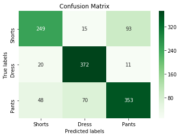
As you can see from the confusion matrix, the result looks pretty decent. Possible next moves may be to test out different network architectures, look at different labels, add more examples from other datasets, and look at using different losses and optimizers to aid in the training. The overall accuracy of the testing data was 80% so there is some room to improve, but the results are much better than the previous post.
The confusion matrix does confirm the issue with the pants and shorts as there are 93 misclassifications for pants and shorts. If feel that the majority of the classification errors may come from the data mainly as it is subjective as to what a pair of shorts are and what are short pants. To overcome this issue, a better data separation technique should be made to be more strict as to what should and should not be classified as pants and shorts.

References:

Hazewinkel, Michiel, ed. (2001) [1994], "Binomial distribution", Encyclopedia of Mathematics, Springer Science+Business Media B.V. / Kluwer Academic Publishers, ISBN 978-1-55608-010-4