ユニファ開発者ブログ

ユニファ株式会社プロダクトデベロップメント本部メンバーによるブログです。

ルクミーフォトリニューアルにおけるデザインワーク

5月に入社したデザイナーのYogaif:id:unifa_tech:20191209181205p:plainです。

この↑アイコンはプライベートの友人が描いてくれました:) 似ているらしい…

今日はルクミーフォトのリニューアルプロジェクトについて、デザイナー視点でざっくり書いてみようと思います。

  • ユニファのデザイナーってどんなことをしているの?
  • 事業会社のインハウスデザイナーってどんなことをしているの?

というようなことに興味のある方はおつきあいください:)

今回の記事で書いていること

  • ルクミーフォトについて
  • リニューアルプロジェクトの進み方とデザイナーの役割
  • 実際の管理画面

ルクミーフォトについて

ルクミーフォトはIoTを使った保育施設向けのフォトサービスです。

プロダクトとしては大きく分けて2つあり、社内ではそれぞれ園管理画面・保護者画面と呼んでいます。

園管理画面
園管理画面:保育園職員が、撮影した写真をアップロードしたり販売設定したりするWebサイト。PCブラウザ

保護者画面
保護者画面:園児の保護者が、園で撮影された写真を閲覧したり購入したりするWebサイト。PCブラウザ・スマートフォンブラウザ

この両方を2018年〜2019年にかけてフルリニューアルしました。

続きを読む

Swift-Jupyter をつかってみました

はじめに

こんにちは、iOSエンジニアのしだです。UniFa Advent Calendarで、普段の開発であまり関わりの少ないメンバーの記事を見てにやにやしてます 😏

こちらは、UniFa Advent Calendar 2019 の12日目の記事になります。

もう2019年が終わりますが、今年は、TensorFlow Dev Sumit 2019があったり、TensorFlow 2.0になったり、O'Reilly主催のTF World '19があったりTensorFlowのアップデートが多かった気がします。 その中で、以下の Swift for TensorFlow (TF World '19) の動画を見ていたところ、何やら Jupyter notebook に Swift を書いていてなんじゃこりゃと思って調べてみたらSwift-Jupyterというものを知ったので使ってみます。

続きを読む

The Pi with Eyes

By Matthew Millar Research Scientist at ユニファ

Purpose:

This blog will cover the progress of an IoT project for computer vision. The final goal will be to locate an individual and to track this individual to see where they are in a room and to tell if they go near a marked area in the room. This will involve; person detection, tracking, and distance measurements from a Raspberry Pi.
Last time we set up the Pi and got things ready to go.
My 2nd Favorite Pi - ユニファ開発者ブログ

This blog post will look at setting up the Pi so it can stream the video feed from a camera. We will cover how to install OpenCV on the Pi and set up a synchronized camera feed from a special Camera Hat which will be discussed later!

IoT:

The IoT is mainly about connecting everything around us to make a holistic data acquisition system. This means all the data that you create is gathered by sensors and sent to the mother node! Let’s break down IoT.
In a nutshell, IoT is a collection of Node or edge devices that gather data by sampling the world around them. This data can range to a large amount because of the different data that can be collected. It can be temperature and weather data, camera feeds, IR sensors, tablets, refrigerators and appliances, and wearable devices to name a few. This is not a comprehensive list as this list is endless and getting longer every day.

Cameras are one of the most common methods for gathering data in an environment. They can be considered the first edge device that was implemented. The world's first security camera came from a chicken farmer who wanted to see who stole his eggs back in 1933. So, the farmer rigged up a camera (like that 35mm film camera professional (use) and hipster have) and set a trap so when the door to the chicken hut was opened the camera would take a picture. He even went so far to put a tin can to make a noise and have the thief look up at the camera [1]. This was the first recorded instance of a security camera. (Yes, the thief was captured and was found guilty).

OpenCV on Pi:

We will need at least one library for using cameras on the Raspberry Pi. That one will be the most common one to use in computer vision projects, OpenCV. This can be complex to install as the older method

pip install opencv-contrib-python

It does not work well with Opencv4 on some Pis. (I tried and failed). So I had to install it from the source. We will go through the steps one by one to get started.
First things first let us get things ready for OpenCV
Update and upgrade the OS first (just like Linux)

sudo apt-get update && sudo apt-get upgrade

Next, we need cmake installed to build the files later.

sudo apt-get install build-essential cmake pkg-config

And then the I/O packages for images

sudo apt-get install libjpeg-dev libtiff5-dev libjasper-dev libpng-dev

And I/O packages for videos

sudo apt-get install libavcodec-dev libavformat-dev libswscale-dev libv4l-dev
sudo apt-get install libxvidcore-dev libx264-dev

We need the GTX development libraries for OpenCV so let’s get them too

sudo apt-get install libfontconfig1-dev libcairo2-dev
sudo apt-get install libgdk-pixbuf2.0-dev libpango1.0-dev
sudo apt-get install libgtk2.0-dev libgtk-3-dev

And a library for aiding in Matrix Manipulation

sudo apt-get install libatlas-base-dev gfortran

And finally the HDF5 and QT GUI

sudo apt-get install libhdf5-dev libhdf5-serial-dev libhdf5-103
sudo apt-get install libqtgui4 libqtwebkit4 libqt4-test python3-pyqt5

Now with all that installed and ready to go let's make our environment to use OpenCV in

Step 1 get and install pip (if you don’t have it already)

wget https://bootstrap.pypa.io/get-pip.py
sudo python get-pip.py
sudo python3 get-pip.py
sudo rm -rf ~/.cache/pip

Now the virtual environment manager

sudo pip install virtualenv virtualenvwrapper

We will update the bashrc file now with the needed information

vim ~/.bashrc

and then add this to the bottom of the file (adjust as needed but if you followed the above exactly then there should be no adjustments)

# virtualenv and virtualenvwrapper
export WORKON_HOME=$HOME/.virtualenvs
export VIRTUALENVWRAPPER_PYTHON=/usr/bin/python3
source /usr/local/bin/virtualenvwrapper.sh

Exit out of the bashrc file and run source to apply all the changes to the bashrc file

source ~/.bashrc

Finally, we can create a new virtual environment

mkvirtualenv myenv_name -p python3

Activate the environment using

Source /path/to/env/myenv_name/bion/activate

And install some needed dependencies.

pip install "picamera[array]"
pip install numpy

Now we can finally get to installing OpenCV from the source

cd ~
wget -O opencv.zip https://github.com/opencv/opencv/archive/4.1.1.zip
wget -O opencv_contrib.zip https://github.com/opencv/opencv_contrib/archive/4.1.1.zip
unzip opencv.zip
unzip opencv_contrib.zip
mv opencv-4.1.1 opencv
mv opencv_contrib-4.1.1 opencv_contrib

This will get all the code you will need to build and install OpenCV
The next step is to make the swap file larger as if you don’t you will not be able to install OpenCV as it takes up too much room

sudo vim /etc/dphys-swapfile

and change the swap size from 100 to 2048. But later on, you will change it back to 100 as using 2048 can burn out your SD card quickly.

# set size to absolute value, leaving empty (default) then uses computed value
#   you most likely don't want this, unless you have an special disk situation
# CONF_SWAPSIZE=100
CONF_SWAPSIZE=2048

After the install, you will change it back to 100 Stop and start the swap service

sudo /etc/init.d/dphys-swapfile stop
sudo /etc/init.d/dphys-swapfile start

Now go back to your virtual environment to work on it. And then we will start to build and configure OpenCV

cd ~/opencv
mkdir build
cd build
cmake -D CMAKE_BUILD_TYPE=RELEASE \
    -D CMAKE_INSTALL_PREFIX=/usr/local \
    -D OPENCV_EXTRA_MODULES_PATH=~/opencv_contrib/modules \
    -D ENABLE_NEON=ON \
    -D ENABLE_VFPV3=ON \
    -D BUILD_TESTS=OFF \
    -D INSTALL_PYTHON_EXAMPLES=OFF \
    -D OPENCV_ENABLE_NONFREE=ON \
    -D CMAKE_SHARED_LINKER_FLAGS=-latomic \
    -D BUILD_EXAMPLES=OFF ..

What makes this special is that ENABLE_NEON is on so that OpenCV is optimized for the ARM processor.
Now you can run

cmake 

But make sure you are inside the build file use pwd to make sure it is in the directory opencv/build/
Next step after the build is done using the

make -j4

Command to compile the code. The -j4 will make it faster as it will use all 4 cores of the Pi. You can leave off the -j4 to avoid possible race conditions if it freezes during install. This will take a hot minute so get lunch and possibly dinner and come back.
Now you can run

sudo make install
sudo ldconfig

The next step is to change the swap size back in the above steps.

Now we need to make a sym-link from the Opencv to python.

cd /usr/local/lib/python3.7/site-packages/cv2/python-3.7
sudo mv cv2.cpython-37m-arm-linux-gnueabihf.so cv2.so
cd ~/.virtualenvs/cv/lib/python3.7/site-packages/
ln -s /usr/local/lib/python3.7/site-packages/cv2/python-3.7/cv2.so cv2.so

Now if all that worked then you can check to see if it actually worked or not (took me 3 tries so don’t get disheartened).
Activate your virtual environment and run the following commands

Python
>>>Import cv2
>>>Cv2.__version__

The Camera Man:

Now we can turn our attention to building the camera system for the project. Looking at the final goal of the project of distance estimation we will need a synchronized set of cameras. Using two cameras that are calibrated and synchronized can greatly improve the accuracy of distance/depth predictions [2]. The camera kit that I will be using will be the Arducam 5MP Synchronized Stereo Camera Bundle Kit for Raspberry Pi that can be bought from Uctronics [3]. Using this chip will handle all the synchronization issues that come with dual camera feeds.

The Setup:

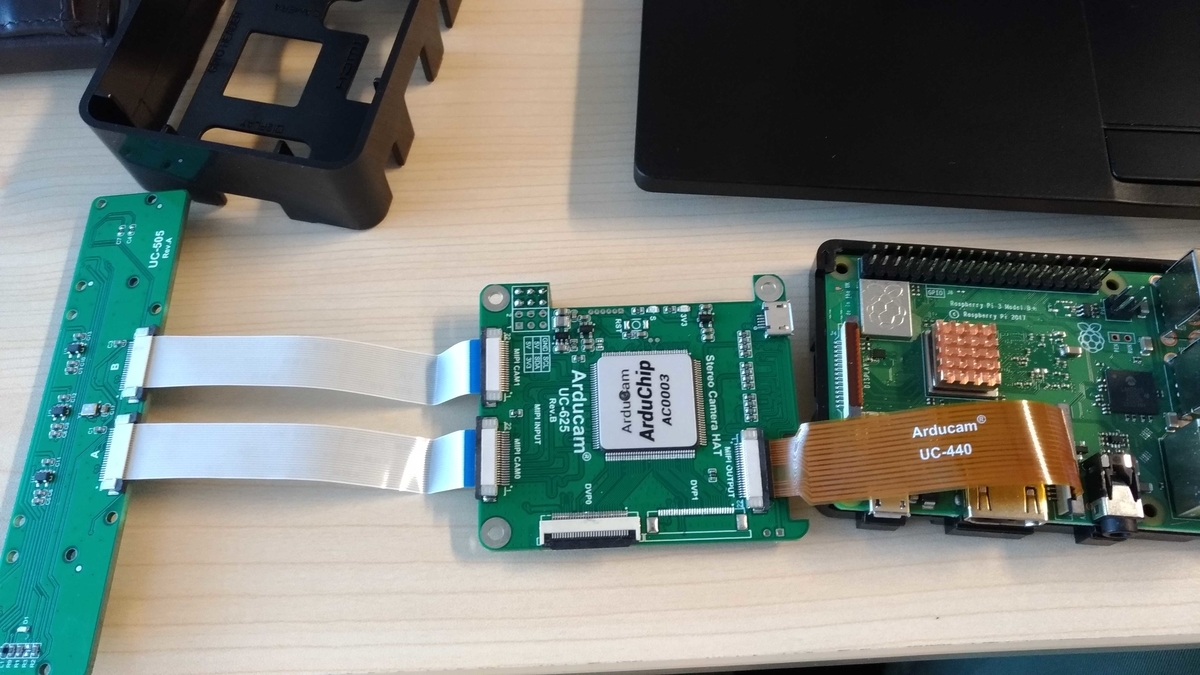
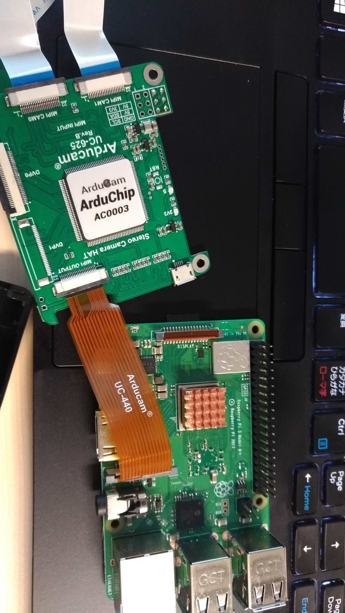
The setup is pretty straight forward. The first step is to connect the ribbon cable from the ArduCam chip to the camera input on the Pi.
f:id:unifa_tech:20191129113459j:plain
f:id:unifa_tech:20191129113515j:plain
Then place the pins into the right connectors on the HAT this will be the topmost pins on the Pi.
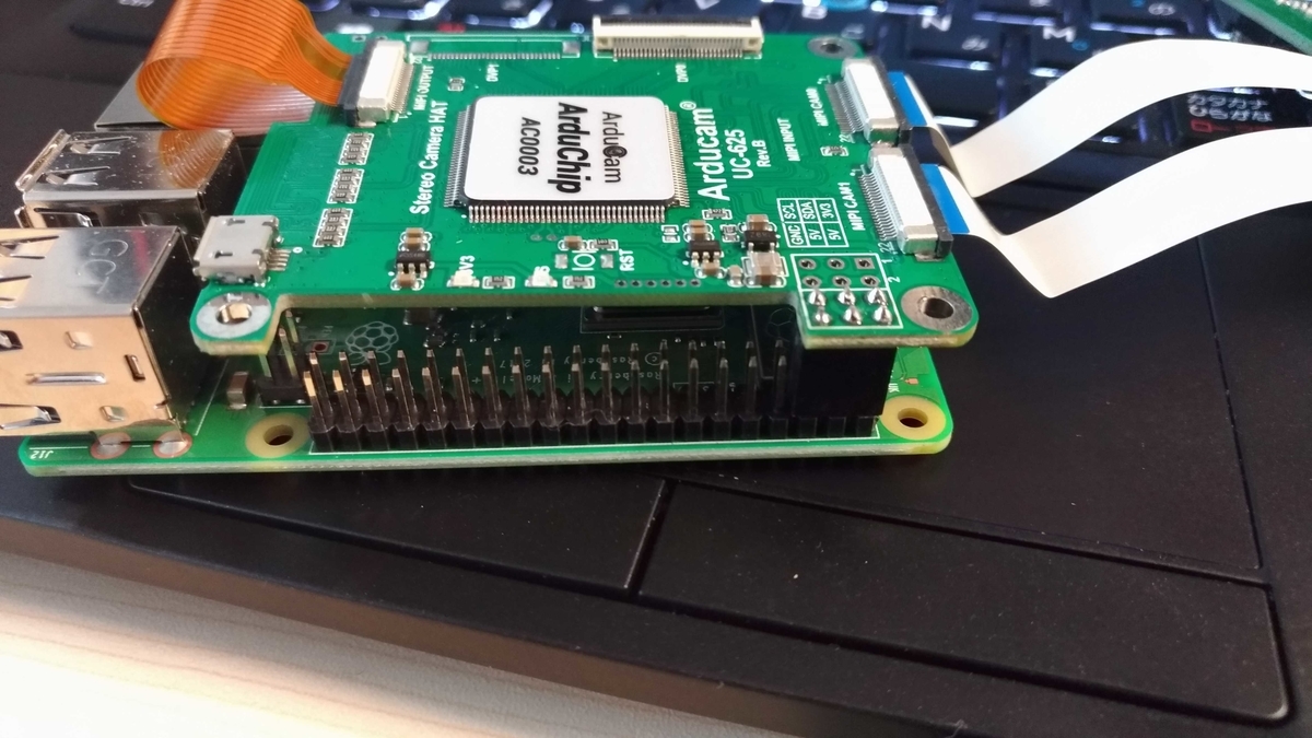
f:id:unifa_tech:20191129113532j:plain
And that's it you are set up and ready to begin installing more packages and dependencies! Let's plug all out stuff in the pi and your setup should look something like this
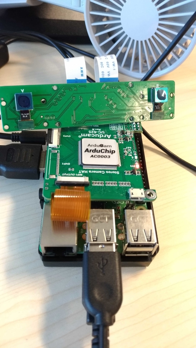
f:id:unifa_tech:20191129113643j:plain
Now even MORE setup and setting changes!
The first step is to enable the camera. On the Pi Desktop go to

Preferences->Raspberry Pi Configuration->Interfaces.

Then Enable the Camera, SSH, VNC, and I2C by clicking the enable radio button. The next step is to download the SKD for the ArduCam chip from GitHub

git clone https://github.com/ArduCAM/MIPI_Camera.git

Go into the RPI folder in the repo and run this command

chmod +x ./enable_i2c_vc.sh
./enable_i2c_vc.sh

This will enable the i2c_vc.
Guess what we need even more Packages again! So run these commands to install them both

sudo apt-get update && sudo apt-get install libzbar-dev libopencv-dev

This will set you up well so you are finally finished installing packages.
The next step is to make the install the code from the repos so do this

cd MIPI_Camera/RPI
make install

Next, compile the examples for testing

make clean && make

And finally, run it in preview mode (a C program from the chips creators).

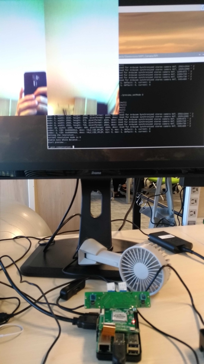
./preview_setMode 0

To actually test out your code. If everything worked out ok you should start to see an image being streamed from the device to your Desktop like this
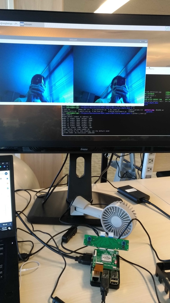
f:id:unifa_tech:20191129113834j:plain
or this
f:id:unifa_tech:20191129113857j:plain

And there you have it you now have an RPi 3B+ with a stereo camera that is synchronized and ready for the next steps.
Next time I will install TensorFlow and start with a simple object detection AI.

Sources:

[1] https://innovativesecurity.com/the-worlds-first-security-camera/

[2] Peleg, S., & Ben-Ezra, M. (n.d.). Stereo panorama with a single camera. Proceedings. 1999 IEEE Computer Society Conference on Computer Vision and Pattern Recognition (Cat. No PR00149). doi: 10.1109/cvpr.1999.786969

[3] https://www.uctronics.com/index.php/arducam-synchronized-stereo-camera-bundle-kit-5mp-for-raspberry-pi-2173.html

ビーコン信号による位置推定(入門)

研究開発部の浅野です。ユニファ2019年アドベントカレンダー10日目の記事は、BLEビーコンを使った位置推定について書きたいと思います。無線信号を活用して位置情報を取得するための方法には様々なアプローチがあります。今回はその中で最もシンプルでわかりやすいビーコン信号強度を利用する方法を紹介します。


構成

ビーコンを活用したサービスは、インドアナビゲーションや近接マーケティングなどのようにビーコン信号を送信(アドバタイズ)する機器が固定されていて移動する人が持つスマホなどでそれを受信する形で応用されていることが多いと思います。しかし、保育園で園児の位置を把握することを考えると、ネットワーク接続が必要になる受信部を壁や遊具に固定して小型の送信装置を園児の名前バッジや衣服などに装着する方が現実的です。

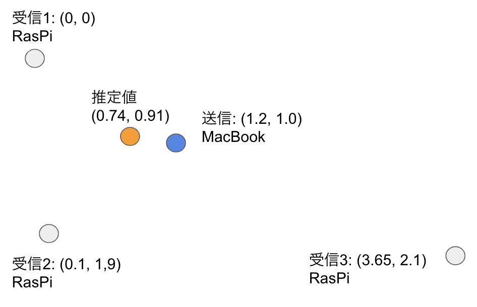
f:id:unifa_tech:20191208112151j:plain:w300:right それを考慮して今回は右のような構成で実験を行います。MacbookからiBeacon信号を送信し、Bluetoothが内蔵されているRaspberry Pi Zero WHを受信装置として3箇所(座標は既知)で信号強度を測定。3つの受信信号強度からそれぞれの距離(d1, d2, d3)を推定してそこからMacBookの位置を割り出します。なお、MacBookからのビーコン信号の送信にはNode.jsのblenoライブラリを使用しました。そして、Raspberry Piでの受信には姉妹ライブラリであるnobleとnobleをバックエンドとして動くnode-beacon-scannerを組み合わせて使いました。


信号強度から距離を推定する

iBeacon受信信号にはTxPowerとRSSI(Received Signal Strength Indication)というフィールドが含まれます。TxPowerはビーコンが発する信号の強さ(実際にはビーコンから1m離れた距離での受信信号強度、単位はdBm)であり、送信側で設定する値です。今回はMacBookから1m離れた地点での実測値(-54.5)を設定しています。一方RSSIは受信した信号の強度(dBm)です。この2つから送信地点と受信地点の距離dを次のように求めることができます(参考)。


d = 10^{\,(TxPower-RSSI)\,/\,(10*n)}

ここで、nはビーコン信号が遮蔽などなく理想的に伝達する空間の場合は2で、通常は環境に応じて最適化する必要があります。今回の実験ではn=2 としています。また、iBeaconはdefaultでは100msごとに信号をアドバタイズしますが、RSSIの値は比較的変動するため各地点とも数秒間の平均をとりました。その結果MacBookと各受信地点との距離(m)は次のように求まりました。


d1 = 1.084, \, d2 = 1.135, \, d3 = 3.055


距離から位置を推定する

各受信地点までの距離が正確に求まる場合は、各地点を中心として半径がそれぞれの距離である円を描くと3つの円が1点で交わります。その点が送信位置です。しかし実際には必ず誤差がのるためそのような幾何的な手法で求めることはできません。そこで、送信位置をxとして、各受信地点との距離の平均二乗誤差を最小にする最適化問題として解いていきます。

import numpy as np

def distance(pos1, pos2): #二点間の距離
    return np.sqrt(sum( (np.array(pos1)-np.array(pos2))**2 ))

def mse(x, locations, distances): #距離の平均二乗誤差
    sum_sqerr = 0.0
    for loc, dist in zip(locations, distances):
        dist_calculated = distance(x, loc)
        sum_sqerr += (dist_calculated - dist)**2
    return sum_sqerr / len(locations)

def midpoint(*args): #中点
    return np.mean(np.array(*args), axis=0)

上のmseが最小にしたい関数です。このように定式化することで受信箇所の数が3より大きい場合にも同様に扱うことができます。最適化問題は例えば下記のようにscipyに含まれるminimize関数を使って解くことができます。

from scipy.optimize import minimize

rec1 = [0, 0]      #受信1の座標
rec2 = [0.1, 1.9]  #受信2の座標
rec3 = [3.65, 2.1] #受信3の座標
d1 = 1.084
d2 = 1.135
d3 = 3.055

locations = [rec1, rec2, rec3]
distances = [d1, d2, d3]
initial_loc = midpoint(locations)

result = minimize(mse, initial_loc, (locations, distances))

f:id:unifa_tech:20191208112229j:plain:w300:right 上のコードで3つの受信地点の座標とそこまでの距離を入力として、距離の平均二乗誤差が最小になる送信地点を求めています。このとき最適化における初期値として3つの受信位置の中点を使っています。この結果求められた送信位置は(0.74, 0.91)でした。正解は(1.2, 1.0)ですのでぴったりではないですがおおよその場所は捉えられています。


まとめ

ビーコンの信号強度を使って送信位置を推定する方法を実装して悪くない結果を得ることができました。今回の実験では送信と受信の間には何も置かず、まわりにもBluetooth機器がそれほどなかったので比較的整った環境でしたが、それでも50cm弱の位置推定誤差になりました。実際の環境では壁、天井、人や物による反射や遮蔽、あるいは他のBluetooth信号との混線などもっとたくさんの誤差要因があります。そういった状況では上述のnの最適化だけでは不十分なことが多く、精度を保つために様々な手法が開発されています。実際のサービスに組み込んでいくためには求められる精度の理解とそれを実現するための必要十分な技術を見極めていくことが重要です。

初めてのre:Invent4日目 (Keynoteとre:Play)

日本に帰ってこんにちは。

時差ボケなのか体力消耗なのか日本に戻って爆睡してしまってた、
ユニファのインフラ見てますすずきです。

今遅ればせながらre:Invent4日目のブログ書いてます。

最終日(re:Invent自体はもう一日ありますが私は最後…)もサクッと認定者ラウンジで朝ごはん食べつつ、
最終日はちゃんと会場でKeynote見ようと会場へ向かいました。

続きを読む

サクッとできるCSSアニメーション(transition)の使い方

Webデザイナーのmorita(こ)です。今回はCSSのアニメーションについて、ちょこっと書かせていただきました。

ボタン(hover me)

↑こんな感じのよくあるhoverアクションを1行で実現します。

 transition: .◯s;

◯の部分は数字でOK。
.4sとかにすると、0.4秒で実行されるアニメーション、
1sとかであれば、1秒で実行されるアニメーションとなります。

※ここ重要!テストに出ます。
【CSS transitionでアニメーションさせるためのポイント】

・対になるプロパティのbefore/afterを用意すること

上記の例だと、

.btn-sample{
  opacity: 1;
  transition: .4s;
}
.btn-sample:hover{
  opacity: 0.3;
}

変化させているプロパティは「opacity(透明度)」なので、beforeは「opacity: 1;(透明度100%)」、afterは「opacity: 0.3;(透明度30%)」です。このあいだの変化を「transition: .4s;(0.4秒)」かけてアニメーションさせています。

例ではCSSでのhoverアクションでしたが、JSなどでの状態変化(clickとかscroll)にもclassを作成して対応できます。(サンプルでは1回しかできません。。)

ボタン(click me)

.move-sample{
  position: relative;
  left: 0;
  transition: .4s;
}
.move-sample.is-anime{
  left: 60%;
}

clickすると、「is-anime」というclassをつけるようにJS書いてもらって、アニメーションのbefore/afterはCSSで制御する感じです。エンジニアとデザイナーが協業で行う時に重宝するやり方です。(JSはトリガーとして、CSSは表現として実装)

transitionの欠点は

・「display: none;」されているとできない。
・ループとできない。

ということです。 上の問題はよくスマホのハンバーガーメニューとかで遭遇しますね。その場合は画面の外に配置したりして、表示する時に画面内に移動してくるとかの対応をしたりしています。 どうしてもこの問題に対応するなら、CSS animationを使うことになります。(その場合、「サクッと」にならないのでググりましょう。)

【他にも色々できちゃったりするよ】
今回はもっとも短く最小のtransitionアニメーションでしたが、他にも様々な設定を指定することが可能です。
transition-property 変化させるプロパティを指定(all,opacity,top/leftなど)
transition-duration 変化させる時間(省略不可、.4sとか秒数を指定)
transition-delay 変化の開始を遅らせる
transition-timing-function イージング(デフォルトはease)

【ブラウザ対応】
IE10以上で実装されているので、ベンダープレフィックスとかもなしでいけるでしょう。

【CSSでアニメーションできる喜び】
少し前まではアニメーションさせるといえば、「JS(jQuery)で」みたいな感じもありましたが、昨今のデザイナーとエンジニアの協業体制を考えると、JSはエンジニア領域、CSSでデザイナー領域として、細部のアニメーションまでを表現(デザイン)できるのが望ましいと感じています。

酔っぱらいの千鳥歩きを参考にしたランダムウォーク メトロポリス・ヘイスティングス法(MH法)を試してみた

はじめに


こんにちわ、研究開発部の島田です。今回はMCMC法の一種である、ランダムウォーク メトロポリス・ヘイスティングス法(MH法)についてのお話です。

これまた小難しそうな名前ですが、実はMCMC法の中では最もシンプルなアルゴリズムとして有名です。今回はこちらを理解した上で実装を行い結果を見てみたいと思います。

おさらい


MH法を理解するにはまずは前回記事の内容が大事になってくるためおさらいをします。

tech.unifa-e.com

前回記事では、マルコフ連鎖について保育士さんの行動モデルを例にして理解しました。 特にある状態が確率的に変化することを遷移核と呼び、マルコフ連鎖を扱うにあたっては非常に重要な概念であることがわかりました。そして、前回記事では遷移核があらかじめわかっている状態でマルコフ連鎖を使いました。しかし、現実問題は遷移核がわからないケースがほとんどであるため、遷移核をどのように設定すればよいのかという問題を解決する必要があります。

遷移核を設定する際に、考えるべきことの一つとしてどのような条件を満たせば定常分布へ収束するのかです。これを詳細つり合いと言い、詳細つり合いを満たすと確率分布が定常分布になります。

そしてこの詳細つり合いをを満たす遷移核は簡単にはわからないため、代わりに条件つき確率分布と乱数によるサンプリング手法を使って、詳細つり合いになるように補正をかけてあげる、これがMH法の考え方になります。乱数によるサンプリング手法については、下記記事を参考にするとイメージがわきやすいです。

tech.unifa-e.com

ランダムウォーク メトロポリス・ヘイスティングス法(ランダムウォークMH法)


前項でも説明した通りMH法の考え方として、詳細つり合いをを満たす遷移核は簡単にはわからないため、サンプリングが簡単な遷移核(提案分布)で代用します。そして詳細つり合いを満たすように提案分布をあとで補正をかけます。

さて、ここで気になるのが、提案分布はどのように決めるのか?ということですね。

よく使われるのがランダムウォークという考え方で、数学や物理学の世界で頻繁に登場します。ランダムウォークという面白い名前なのですが、由来となっているのはなんと酔っ払いの千鳥歩きだそうです。これからの忘年会シーズンでよく目にする酔っ払いがフラフラ歩いている姿、そうあれです。そしてランダムウォークを使ったMH法のことを、ランダムウォークMH法と呼びます。

f:id:unifa_tech:20191203132307p:plain:w300

では、酔っ払いの千鳥歩き(ランダムウォーク)を数学的に表現してみます。まずは一番シンプルな一次元のランダムウォークは下図のように表せます。最初に豚の酔っ払いさんがいる地点から左に行くのか右に行くのかは確率的な問題です。

f:id:unifa_tech:20191206095259p:plain
(豚さんのイラスト 出典: かわいいフリー素材集 いらすとや

新しい地点θnewは下記のように表せます。

θnew = θ + ε Normal(0, 1)

ここで、εはランダムウォークが動く幅を表すパラメータです。Normal(0, 1)は0〜1の正規分布を仮定しています。

さて、ランダムウォークについて理解したところでいよいよランダムMH法の中身について理解していきます。

まずはMH法の一般的な考え方についてですが、先に詳細つり合いを形式化します。

f(θ'|θ)f(θ) = f(θ|θ')f(θ')

左辺については、例えばある確率θが発生します(実際には事後分布)。そうすると、確率θθ'に移ります(遷移核)。右辺は今度はあるθ'が発生して、θ'θに移ることを示しています。詳細つり合いを満たすということはすなわちこれらの確率の流れが等しくなることになります。

MH法では、サンプリングが簡単な提案分布q(θ'|θ)で代用しますが、このとき詳細つり合いは厳密には満たされないために、

q(θ'|θ)f(θ) > q(θ|θ')f(θ')

というような式で表せます。

そこで、詳細つり合いを満たすように補正係数γを導入します。

γq(θ'|θ)f(θ) = q(θ|θ')f(θ')

これをγについて解くと下のようになります。

γ=\dfrac{q(θ|θ')f(θ')}{q(θ'|θ)f(θ))}

すなわち、このγという補正係数を導入することで詳細つり合いを満たすような遷移が実現できることになります。

ここで、ランダムウォークの概念を取り入れると、q(θ'|θ)q(θ|θ')は等しくなるはずです。なぜならば上の一次元ランダムウォーク図を見るとわかる通り、豚さんが右に移動する確率と移動された地点から元の場所に移動する確率も等しいはずですよね。そのため、補正係数γは下記のようにシンプルに表せます。

γ=\dfrac{f(θ')}{f(θ)}

少し説明が長くなりましたが、実際にこのアルゴリズムを実装してみます。

ランダムウォークMH法の実行


今回もベータ分布で確認してみます。まずはベータ分布の確認です。

np.random.seed()
a, b = 1.8, 2.9
x = np.linspace(beta.ppf(0.001, a, b), beta.ppf(0.999, a, b), 100)
plt.plot(x, beta.pdf(x, a, b))
f:id:unifa_tech:20191203134222p:plain:w500

次にランダムウォークMH法のコアな部分ですが、流れとしては下のフローのようになります。

  1. 初期値θを決定する(適当で良い)

  2. ランダムウォークを使って次の新しいθ’を探索

  3. 次の条件式の判定。f(θ) > f(θ')

  4. Step3の条件式が、

 ・真の場合、現在位置の方が次の位置よりも確率分布の高い位置であると言えるため、γで補正する。区間[0, 1]の一様乱数を生成し、γと比べて小さい場合は受理、それ以外の場合は棄却する。

 ・偽の場合、補正せずに新しい乱数を受理する。

これを実装して、結果を確かめてみます。

def rw_MH():
    NUM_MC_STEP = 30000#モンテカルロステップ数
    theta = 0.6#ランダムウォークの初期値
    E = 0.5#ランダムウォークの幅
    theta_mc_step = [theta]
    
    for i in range(NUM_MC_STEP):
        re_theta = theta + E * np.random.randn()
        if beta.pdf(theta, a, b) > beta.pdf(re_theta, a, b):
            gamma = beta.pdf(re_theta, a, b) / beta.pdf(theta, a, b)
            if np.random.rand() < gamma:
                theta = re_theta
        else:
            theta = re_theta
        theta_mc_step.append(theta)
    
    return theta_mc_step
f:id:unifa_tech:20191203135203p:plain:w500

オレンジ色の曲線が元のベータ分布ですが、ランダムMH法によるサンプリングも同じような曲線が得られていることがわかります。

最後に


今回はMCMC法の最もシンプルなランダムウォークMH法を理解し、実装・結果を見てみました。遷移核があらかじめわかっていないケースにおいてもサンプリングが可能になりました。他にもギブスサンプラーやハメルトニアンモンテカルロ法といった様々なMCMC法があるので、是非今後も試してみたいと思います。

参考文献


・RとStanではじめるベイズ統計モデリングによるデータ分析入門(講談社)

基礎からのベイズ統計学 輪読会資料 第4章 メトロポリス・ヘイスティングス法